Assimilating Almost Anything into Almost Any Stochastic Model
Lachlan Astfalck
UNSW Sydney | STREAM

What are we trying to do?
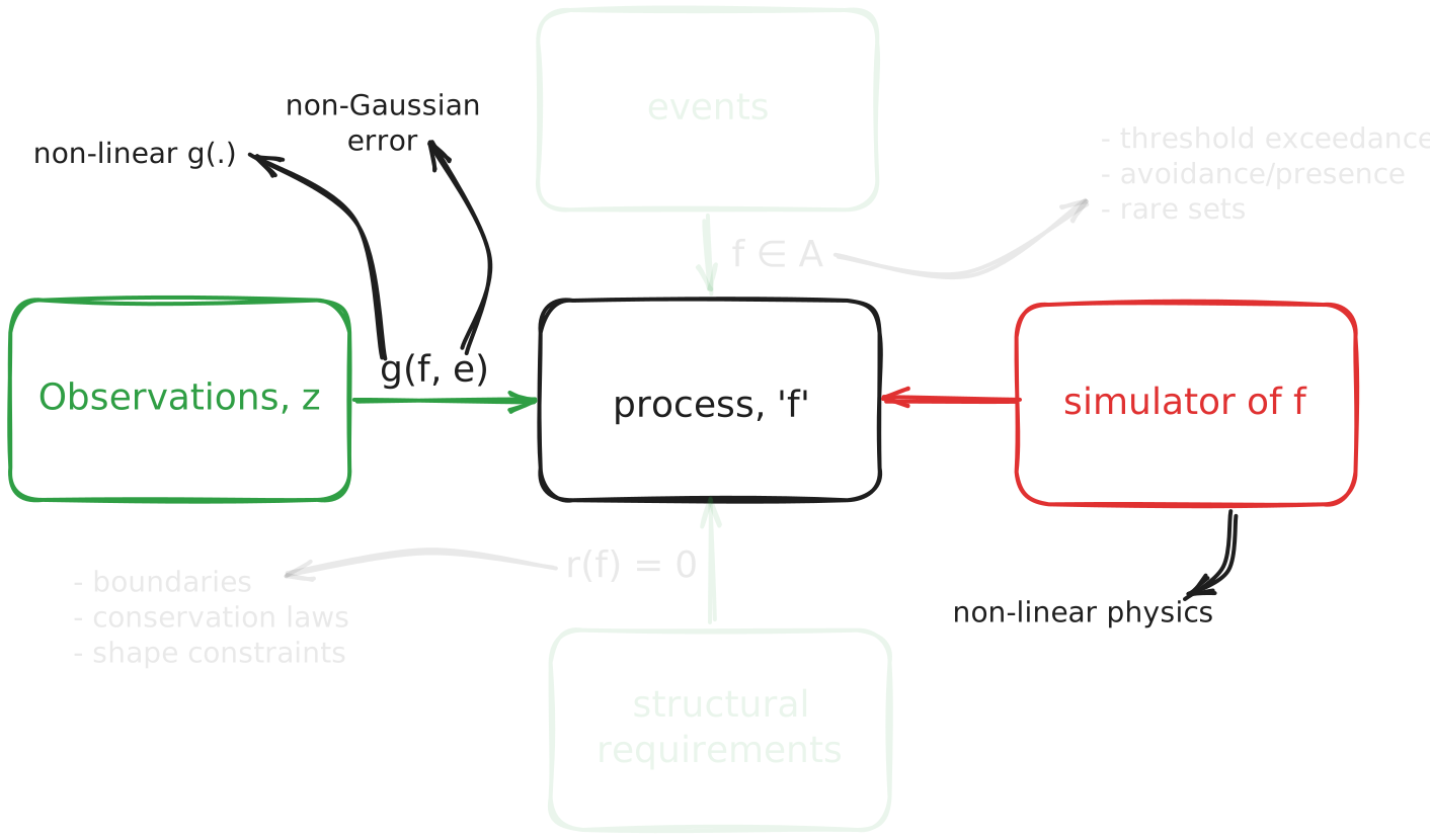
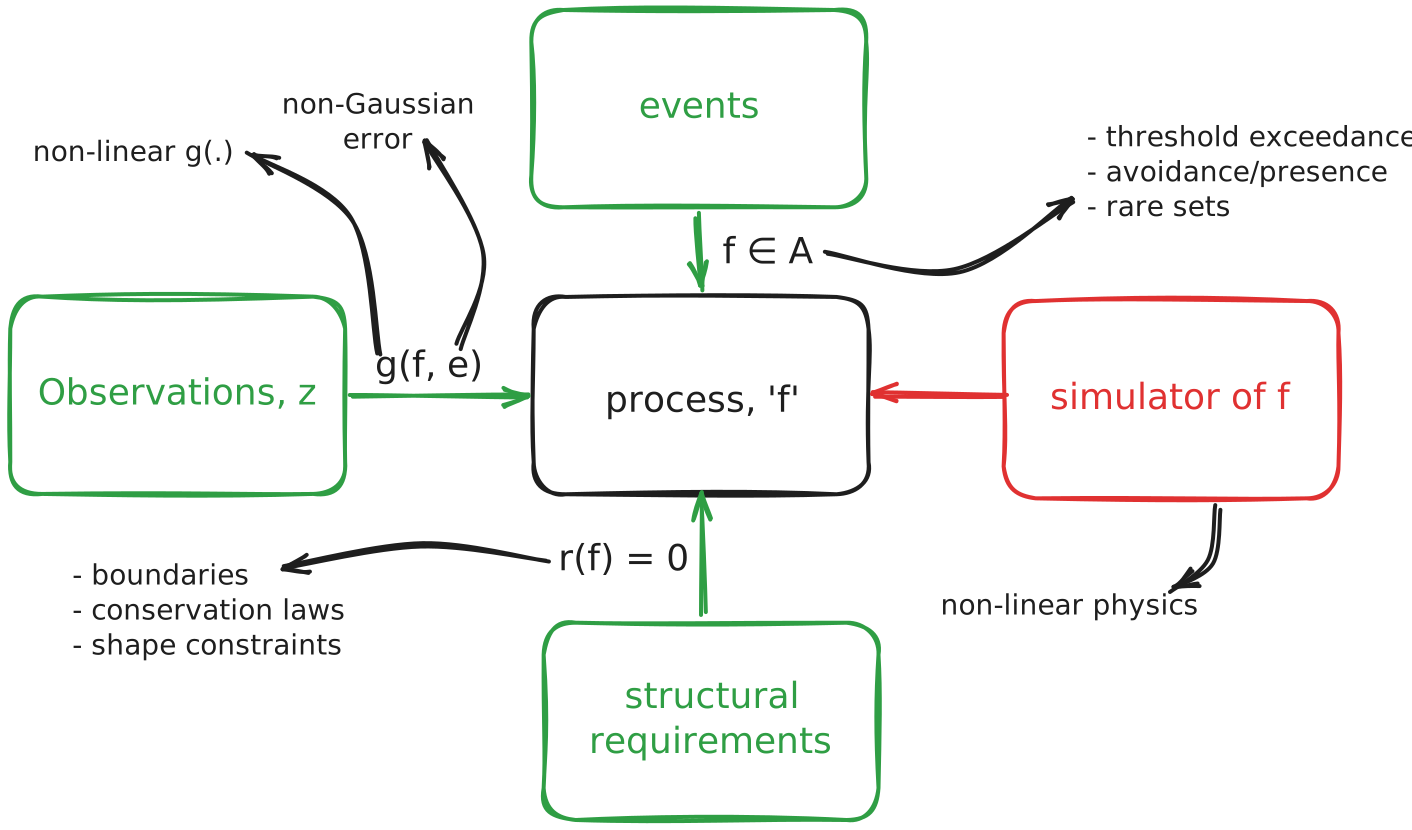
- Take a stochastic model you can run forward: a solver, a stochastic parameterisation, a field simulator. Call it a stochastic process \(f\).
- We want runs that assimilate/agree with some information \(\mathcal{C}\):
- sparse, indirect, bounded-below observations — gauges, satellite retrievals, floats;
- a budget or a boundary condition the analysis has to respect;
- an event we want to impose — a heatwave of a given severity, a surge above a given level.
- Working assumption: running the unconditional model forward is easy, steering/conditioning is hard.
We are targeting the quantity \(p(f \mid \mathcal{C})\).
Some Nomenclature
- Field - some general notion of a latent/unobserved/incomplete physical process
- Assimilation - incorporating information into your field
- Model - some structured belief on your field (not necessarily a numerical model)
- Stochastic Model - any structured belief with some formal mechanism that may be perturbed
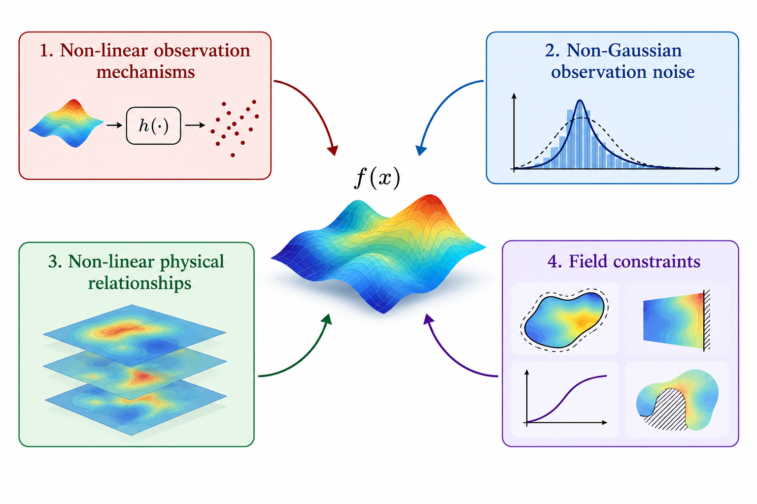
Data Assimilation (the noun)
| prior | observation model | what you get | |
|---|---|---|---|
| OI / 3D-Var | Gaussian, static \(\mathbf{B}\) | linear \(H\), Gaussian | a mean and a covariance |
| 4D-Var | Gaussian, model as strong constraint | linearised \(H\), Gaussian | the mode, via the adjoint |
| EnKF | an ensemble, Gaussian in the update | linear update | a shifted ensemble |
| this talk | your model \(f\) | almost anything | draws from the true posterior |
All Cats Are Stochastic Processes
A cat is a random vector
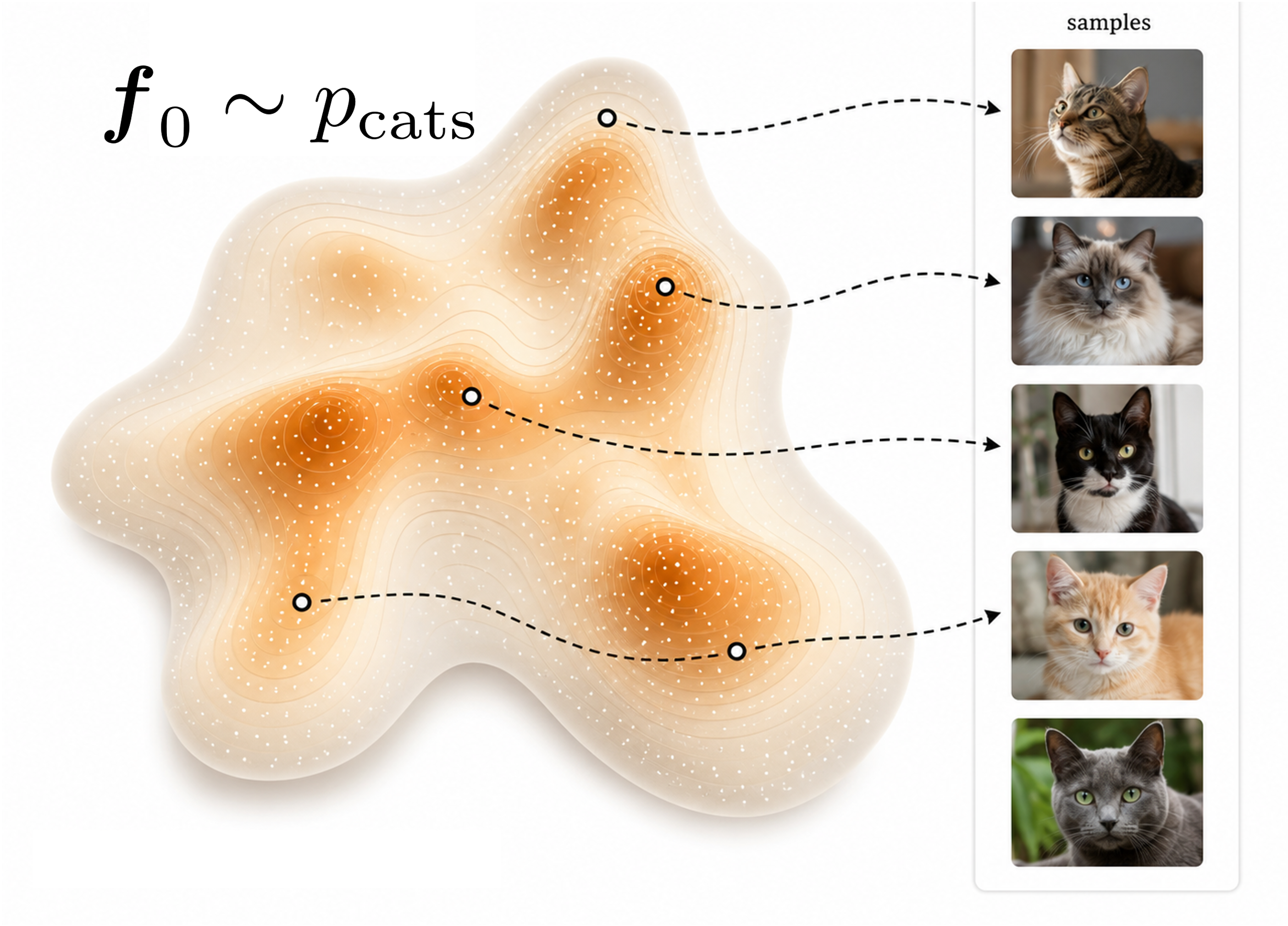
Diffusion modelling simply asks “how do I sample from an inconvenient distribution?”
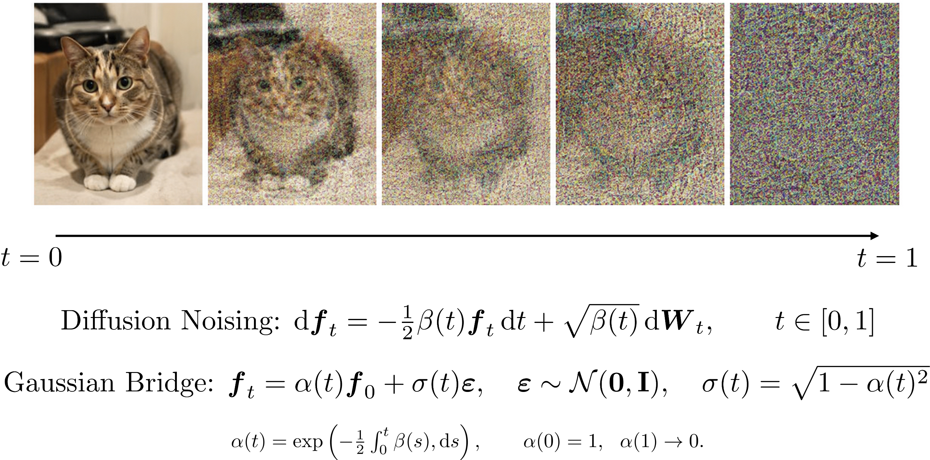
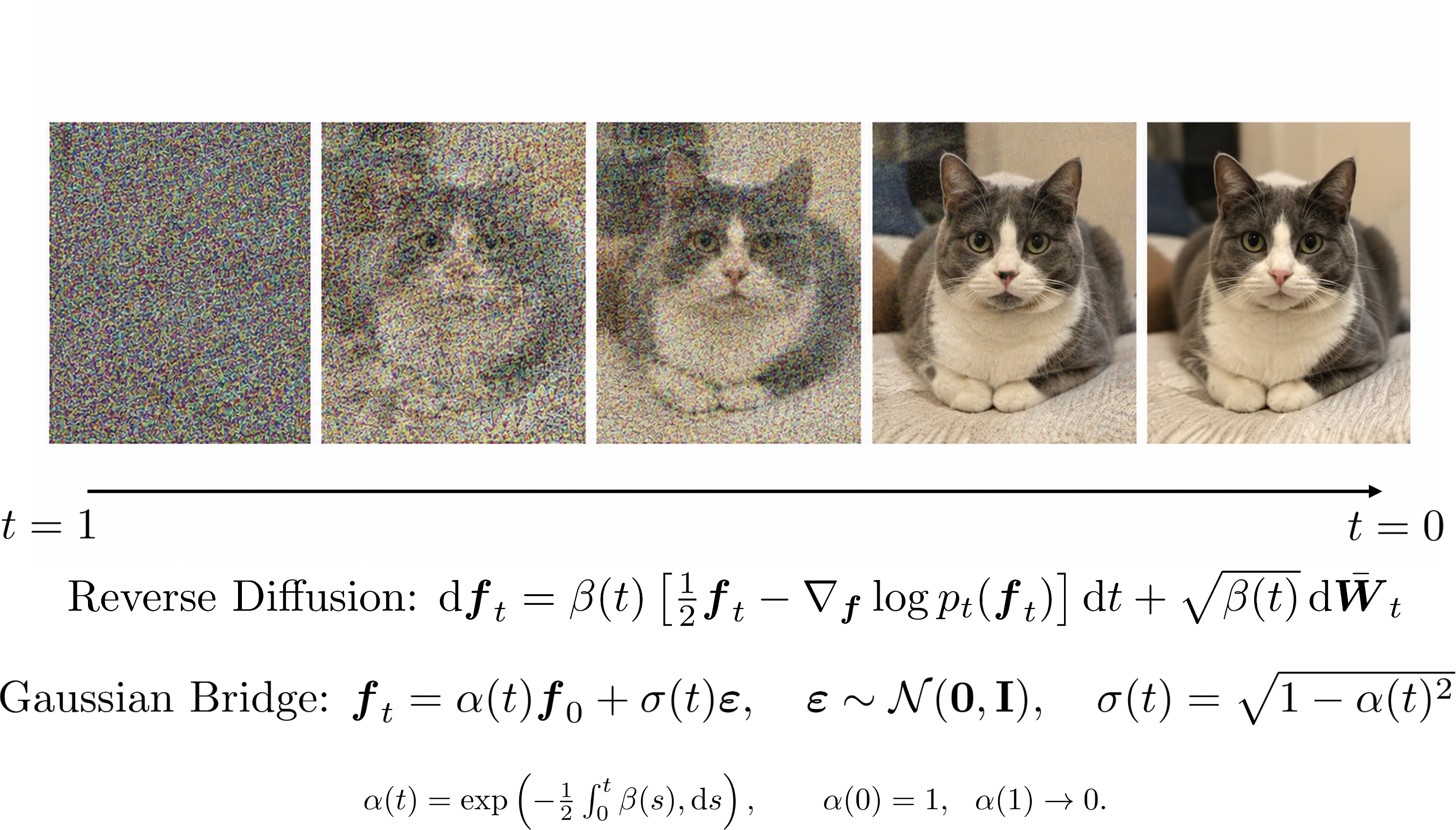
Noising a cat
Reversing a cat
- Write \(p_t\) for the marginal of \(\boldsymbol{f}_t\) — the law of the process after noising for time \(t\)
- (so \(p_0 = p_\text{cat} = \mathcal{SP}\), \(p_1 \approx \mathcal{N}(\boldsymbol{0}, \mathbf{I})\))
- Anderson (1982) showed that the time reversal is also an SDE, \[\begin{aligned} \text{Forwards:}& \qquad \mathrm{d}\boldsymbol{f}_t = - \tfrac{1}{2}\beta(t) \boldsymbol{f}_t \mathrm{d}t + \sqrt{\beta(t)}\,\mathrm{d}\boldsymbol{W}_t. \\ \text{Backwards:}& \qquad \mathrm{d}\boldsymbol{f}_t = \beta(t)\left[\tfrac{1}{2}\boldsymbol{f}_t - \nabla_{\boldsymbol{f}}\log p_t(\boldsymbol{f}_t)\right]\mathrm{d}t + \sqrt{\beta(t)}\,\mathrm{d}\bar{\boldsymbol{W}}_t. \end{aligned}\]
- One unknown object: the time-dependent score \(\nabla_{\boldsymbol{f}} \log p_t\).
- If we know the score, noise flows backwards into cats.
Anderson (1982), Reverse-time diffusion equation models, Stochastic Processes and their Applications 12(3):313–326.
Reversing a cat
Google’s GenCast
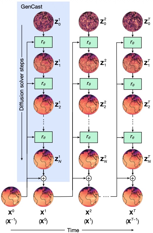
Price, Ilan, et al. (2025), Probabilistic weather forecasting with machine learning., Nature 637(8044): 84-90.
What does machine learning do?
- For cats, \(\nabla_\boldsymbol{f} \log p_t\) is unknown. Diffusion models learn it by fitting a network \(s_\theta(\boldsymbol{f}, t)\).
- That is the entire “ML” content of a diffusion model; everything else is stochastic calculus.
- find a few hundred million photographs of cats;
- noise every one of them along the forward process;
- train \(s_\theta(\boldsymbol{f}, t) \approx \nabla_\boldsymbol{f} \log p_t\) on the pairs;
- sample from \(p_\text{cats}\) by pushing white noise through the reverse SDE.
Conditional cats
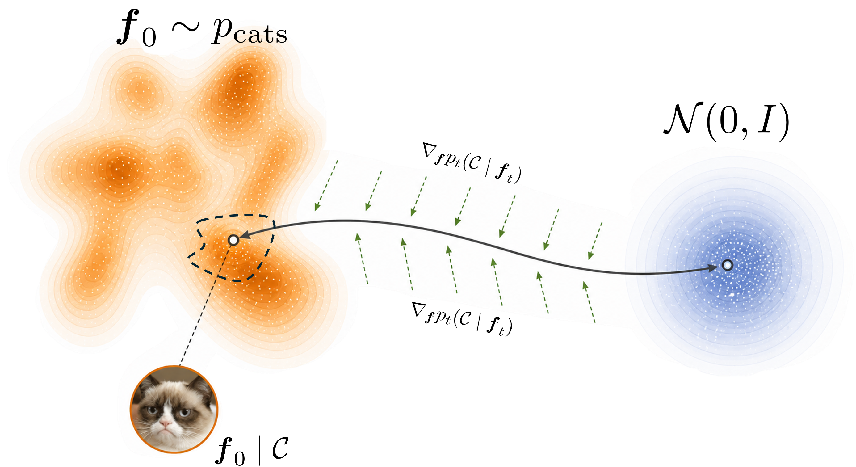
- Want a grumpy cat? Bayes: \[ \nabla \log p_t(\boldsymbol{f}_t \mid \mathcal{C} = \text{grumpy}) = \nabla \log p_t(\boldsymbol{f}_t) + \underbrace{\nabla \log p_t(\mathcal{C} = \text{grumpy} \mid \boldsymbol{f}_t)}_{\text{the pull towards } \mathcal{C}}. \]
- Add a likelihood term to the drift and the trajectory bends towards draws satisfying \(\mathcal{C}\): \[\mathrm{d}\boldsymbol{f}_t = \beta(t)\left[\tfrac{1}{2}\boldsymbol{f}_t - \nabla_{\boldsymbol{f}}\log p_t(\boldsymbol{f}_t \mid \mathcal{C})\right]\mathrm{d}t + \sqrt{\beta(t)}\,\mathrm{d}\bar{\boldsymbol{W}}_t.\]
- Machine learning calls this guidance. It is Bayes’ rule added to a drift.
Conditional cats
Stoch. Models Are Boring Cats
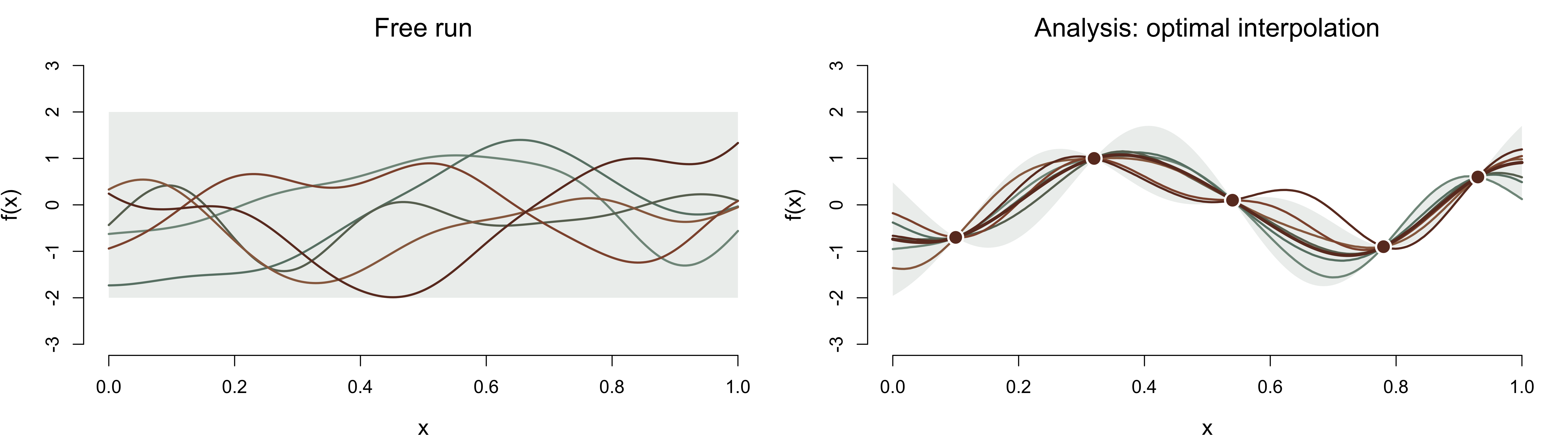
Gaussian Processes / Kriging / OI
- A Gaussian process is a distribution over fields: any finite set of locations has a joint normal distribution with covariance \(k(x,x')\).
- With linear Gaussian observations \(\boldsymbol{y} = \mathbf{L}\boldsymbol{f}_0 + \boldsymbol{\varepsilon}\), the posterior mean is closed form, \[ \mathbf{m}_{*|\boldsymbol{y}} = \mathbf{m}_* + \mathbf{K}_{**}\mathbf{L}^{\mathsf{T}}\!\left(\mathbf{L}\mathbf{K}_{**}\mathbf{L}^{\mathsf{T}} + \boldsymbol{\Gamma}\right)^{-1}\!(\boldsymbol{y} - \mathbf{L}\mathbf{m}_*). \] This is optimal interpolation, with \(\mathbf{K}_{**} \equiv \mathbf{B}\).
Targeting a GP with a Diffusion
The marginal \(p_t\) stays Gaussian, and we know \[ p_t = \mathcal{N}\big(\boldsymbol{b}(t),\, \mathbf{A}(t)\big), \qquad \boldsymbol{b}(t) = \alpha(t)\,\mathbf{m}_*, \qquad \mathbf{A}(t) = \alpha^2(t)\mathbf{K}_{**} + (1-\alpha^2(t))\mathbf{I}. \]
So the score is closed form, and no network is required:
\[ \nabla_{\boldsymbol{f}}\log p_t(\boldsymbol{f}_t) = -\mathbf{A}(t)^{-1}\big(\boldsymbol{f}_t - \boldsymbol{b}(t)\big). \]
Drop it into the reverse-time SDE and integrate from \(t=1\) to \(t=0\):
\[ \mathrm{d}\boldsymbol{f}_t = \beta(t)\left[\tfrac{1}{2}\boldsymbol{f}_t - \nabla_{\boldsymbol{f}}\log p_t(\boldsymbol{f}_t)\right]\mathrm{d}t + \sqrt{\beta(t)}\,\mathrm{d}\bar{\boldsymbol{W}}_t. \]
A GP/OI is a very boring cat with a score we can write down.
Watch it happen
Whitening into better coordinates
“The most efficient thing for a computer to do is nothing” - Prof. Philipp Hennig
Whiten: \(\hat{\boldsymbol{f}}_0 = \mathbf{K}_{**}^{-1/2}(\boldsymbol{f}_0 - \mathbf{m}_*)\), the dynamics vanish entirely … the linear drift term is zero.
Your model is already the generator
- A draw from the process is a deterministic map of simple noise: \[ \boldsymbol{f}_0 = T_\vartheta(\boldsymbol{\xi}_0), \qquad T_\vartheta : \mathbb{R}^{m} \to \mathbb{R}^{d}, \qquad \boldsymbol{\xi}_0 \sim \mathcal{N}(\boldsymbol{0}, \mathbf{I}_m). \]
- For a Gaussian field, \(T_\vartheta\) is the Cholesky factor. For an SDE or an SPDE, \(T_\vartheta\) is the integrator and \(\boldsymbol{\xi}_0\) are its driving increments.
- Run the diffusion in \(\boldsymbol{\xi}\), where the prior is standard normal and the score is exactly \(-\boldsymbol{\xi}_t\), then push through \(T_\vartheta\).
- Rosenblatt (1952): after discretisation, every process admits such a representation.
Rosenblatt (1952), Remarks on a multivariate transformation, The Annals of Mathematical Statistics 23(3):470–472.
A gallery of boring cats
Every one is \(\boldsymbol{f}_0 = T_\vartheta(\boldsymbol{\xi}_0)\) for a tractable generator \(T_\vartheta\) and iid-normal latent \(\boldsymbol{\xi}_0\):
- Gaussian and heavy-tailed fields — the usual spatial priors, plus tails that match precipitation and surge: a Gaussian draw times a scale or mixing variable.
- Categorical fields — sea ice, land cover, cloud regime: ordered labels read off latent noise (e.g. a Potts model).
- SDEs/SPDEs — stochastic physics parameterisations, energy-balance and box models: \(T_\vartheta\) is the Euler-Maruyama step and \(\boldsymbol{\xi}_0\) are its increments.
- “Stochastic” numerical models — WRF, MOM, ROMS, a Lagrangian particle tracker, …
Where we stand
- Push \(\boldsymbol{\xi}_0 \sim \mathcal{N}(\boldsymbol{0},\mathbf{I})\) through \(T_\vartheta\)
- This gives marginal samples of nearly any stochastic process. (We could already do this, it’s just simulation.)
- The score of the latent noising process with respect to \(\boldsymbol{\xi}_t\) is closed form.
- Thus the boring-cat property survives in latent space for every process in the gallery.
- Now we need a framework for conditioning…
Sneak Peak - Physics as conditioning information
\[ \nabla \log p_t(\boldsymbol{f}_t \mid \mathcal{C}) = \nabla \log p_t(\boldsymbol{f}_t) + \nabla \log p_t(\mathcal{C} \mid \boldsymbol{f}_t). \]
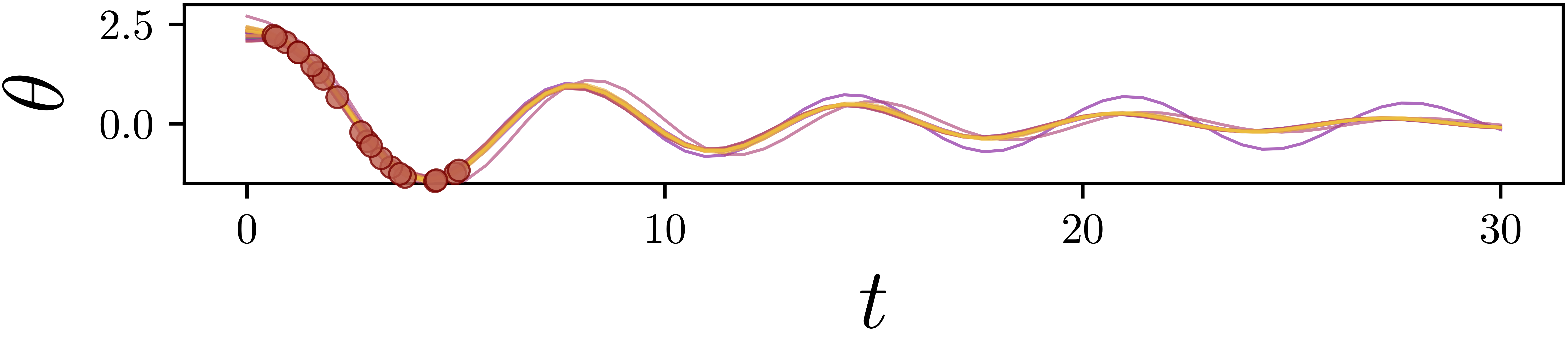
Optimal interpolation, conditioned on the observations alone
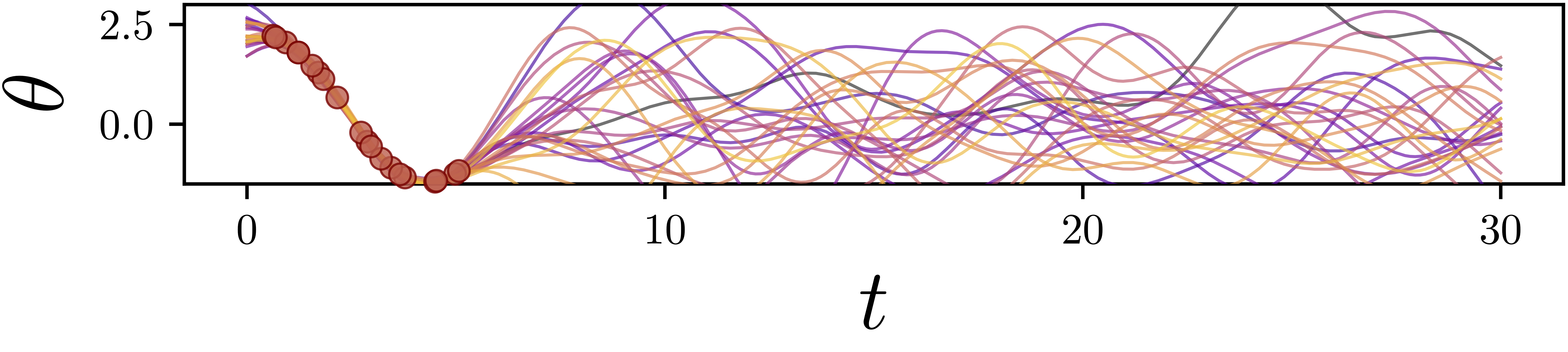
Conditioned on the observations and on the non-linear damped pendulum equation
Grumpy Stochastic Models
Guidance is just Bayes
We work in latent space. Target the pulled-back posterior: \[ \pi(\boldsymbol{\xi}_0 \mid \mathcal{C}) \propto p\big(\mathcal{C} \mid T_\vartheta(\boldsymbol{\xi}_0)\big) \rho(\boldsymbol{\xi}_0). \]
Along the latent flow, the score decomposes: \[ \nabla_{\boldsymbol{\xi}} \log p_t(\boldsymbol{\xi}_t \mid \mathcal{C}) = \underbrace{\nabla_{\boldsymbol{\xi}} \log p_t(\boldsymbol{\xi}_t)}_{=\,-\boldsymbol{\xi}_t\ \text{(exact)}} + \underbrace{\nabla_{\boldsymbol{\xi}} \log p_t(\mathcal{C} \mid \boldsymbol{\xi}_t)}_{\text{guidance}}. \]
Run the same SDE in \(\boldsymbol{\xi}\)-space, add the guidance term, then push through \(T_\vartheta\).
The latent prior is exact at every \(t\). Guidance is the only thing to approximate.
Guidance, in practice
The increment is the pull towards \(\mathcal{C}\), averaged over where the current draw could still end up: \[ \nabla_{\boldsymbol{\xi}}\log p_t(\mathcal{C}\mid \boldsymbol{\xi}_t) \approx \alpha(t) \sum_{i=1}^{S} \bar{w}^{(i)}\, \nabla_{\boldsymbol{\xi}}\log p\big(\mathcal{C}\mid T_\vartheta(\boldsymbol{\xi}_0^{(i)})\big), \qquad \bar w^{(i)} \propto p\big(\mathcal{C}\mid T_\vartheta(\boldsymbol{\xi}_0^{(i)})\big). \]
- For us, guidance is a Monte Carlo average.
- Each term is one gradient of the observation model, pulled back through the model: \[ \nabla_{\boldsymbol{\xi}}\log p\big(\mathcal{C}\mid T_\vartheta(\boldsymbol{\xi}_0)\big) = \underbrace{\big[\partial_{\boldsymbol{\xi}} T_\vartheta(\boldsymbol{\xi}_0)\big]^{\!\mathsf T}}_{\text{Jacobian of the integrator}}\, \nabla_{\boldsymbol{f}_0}\log p(\mathcal{C}\mid\boldsymbol{f}_0). \]
- No training set, no MCMC, no bespoke derivation for each new \(\mathcal{C}\).
(There are known weight-degeneracy issues in importance sampling that do not appear to matter here, for a handful of esoteric reasons.)
The model derivative
- You need \(\partial_{\boldsymbol{\xi}} T_\vartheta\): the derivative of the integrator with respect to its own random draws. This is the same class of object 4D-Var needs, obtained by autodiff through the solver.
- NeuralGCMs are the existence proof that a serious climate model can be written this way.
- Unlike 4D-Var, the output is draws from the posterior, so you can compute any functional you like and honest uncertainty comes free.
- Unlike 4D-Var and the EnKF, the observation model may be non-Gaussian, bounded, censored, or an inequality.
- Where the code is not differentiable there are some sneaky tricks that we can do.
A Computational Caveat
- We are not cheapening a hard computation. An expensive model is expensive to condition.
- Cost per posterior draw \(\approx\) \(\mathcal{O}\)(reverse-SDE steps) forward model integrations.
- Ensemble members can be generated in parallel.
- Where a model is prohibitively expensive, we may still use an emulator, but this is a matter of practicality not feasibility.
| Error source | Image diffusion | Simulator-based | |
|---|---|---|---|
| 1 | Marginal score \(\nabla\log p_t\) | uncontrolled | exact |
| 2 | Guidance approximation | uncontrolled | explicit; \(\mathcal{O}(S^{-1})\) bias |
| 3 | Discretisation | controllable | solver order \(h^q\), same bound |
When do neural networks still help?
- Our thesis so far: if you can simulate, the score is free and the network goes away
- This does nothing for computation
- A generative emulator may still be helpful to enable computation
- A NN provides an adjoint. An emulator is differentiable by construction; forty years of Fortran is not.
- A learned emulator might account for model misspecification (e.g. GenCast vs ENS)
The conditioning mechanism does not care where the score comes from. Closed form from your solver, or learned from data.
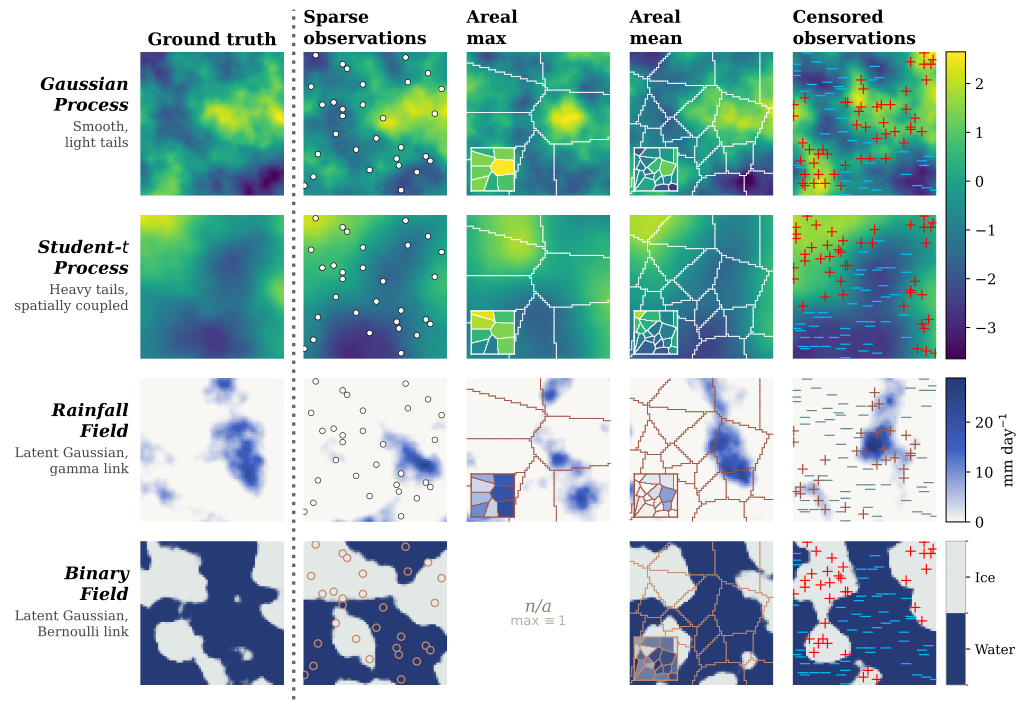
Spatial fields, awkward observations
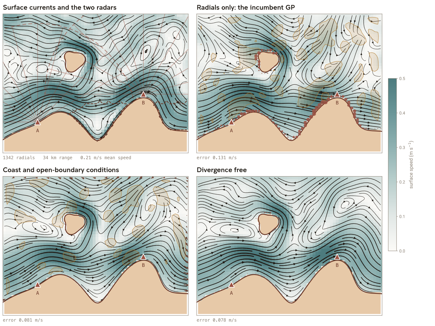
HF Radar Currents with known Boundaries
A toy land–atmosphere feedback model
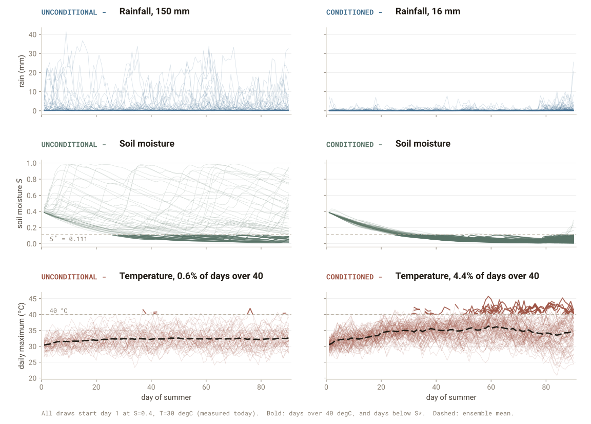
\[ \mathrm{d}T = -\kappa(S)\,\bigl(T - T^{*}(S)\bigr)\,\mathrm{d}t + \sigma_T\,\mathrm{d}W_T, \qquad \mathrm{d}S = 1/C_S \bigl(P(t) - E(T,S)\bigr)\,\mathrm{d}t \]
\(\kappa(S)\) relaxation rate · \(T^{*}(S)\) equilibrium temperature · \(C_S\) soil water storage capacity · \(P(t)\) precipitation · \(E(T,S)\) evaporative water loss
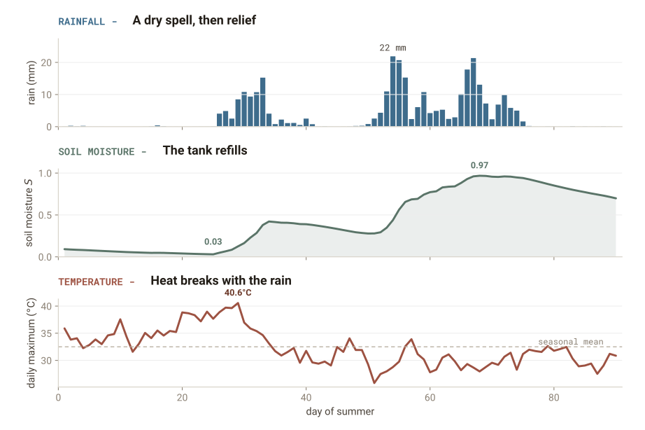
An insultingly simplified version of Brubaker & Entekhabi (1996).
A toy land–atmosphere feedback model
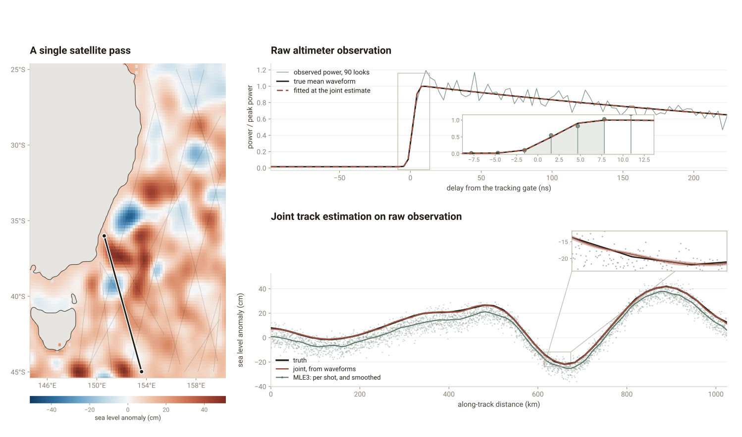
Spatio-temporal SPDEs
SSH from Altimetry “Data”
Methane Flux Inversion
NN + Diffusion based inversion of methane flux

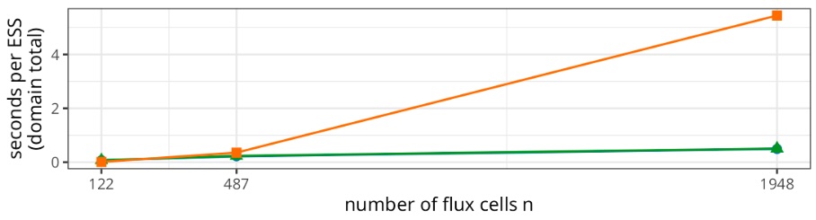
Computational scaling vs true-model inversion
Conditioning on Natural Language
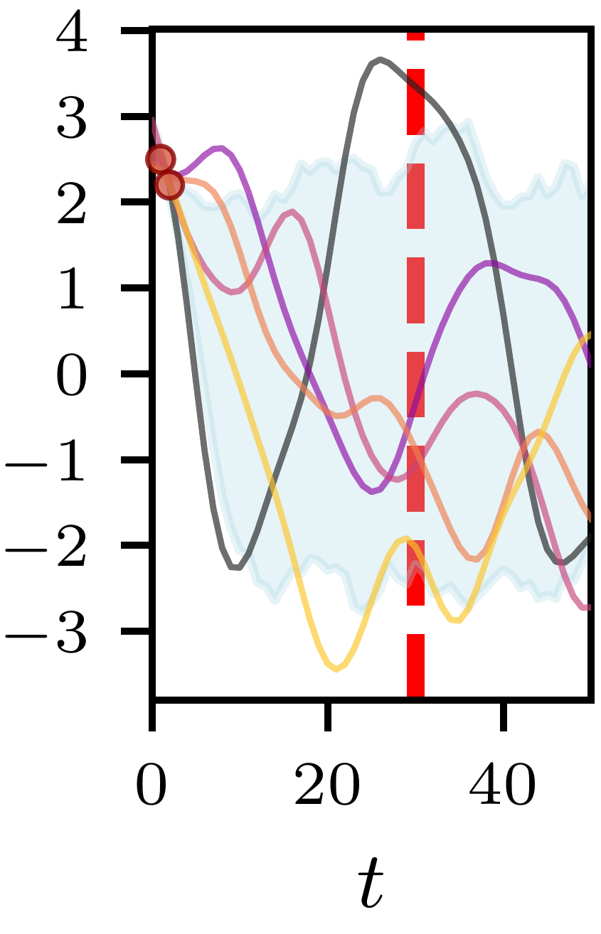
“A small UK company’s daily stock price in GBP over 50 trading days. On day 30 the company enters compulsory liquidation and is permanently delisted from the London Stock Exchange.”
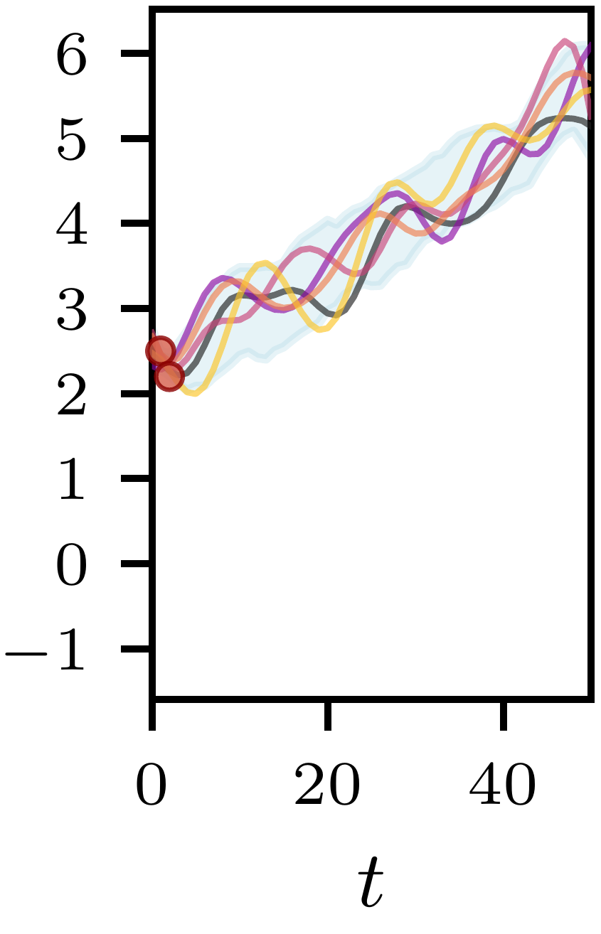
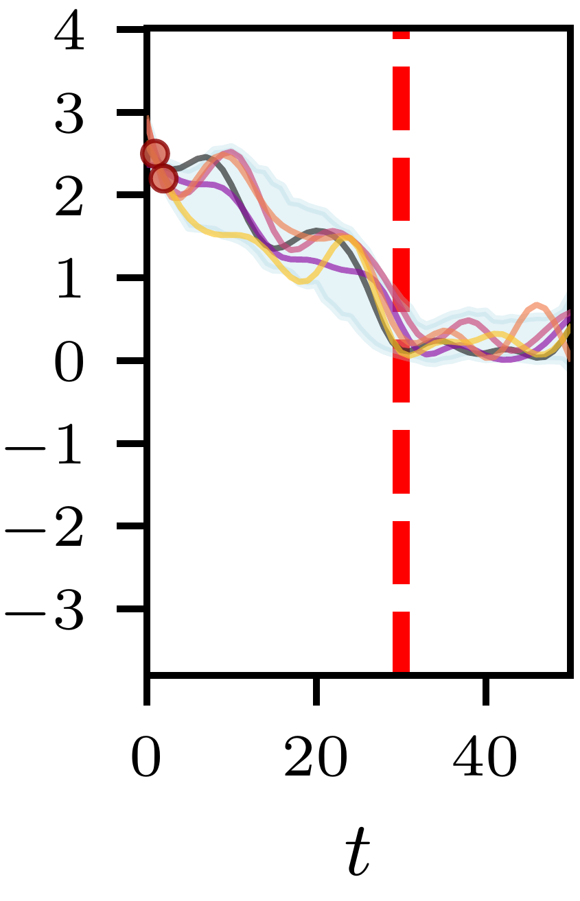
“A small UK company’s daily stock price in GBP over 50 trading days. The company has no notable news during the period, but performs well. Ending with a value over 5 GBP per share.”
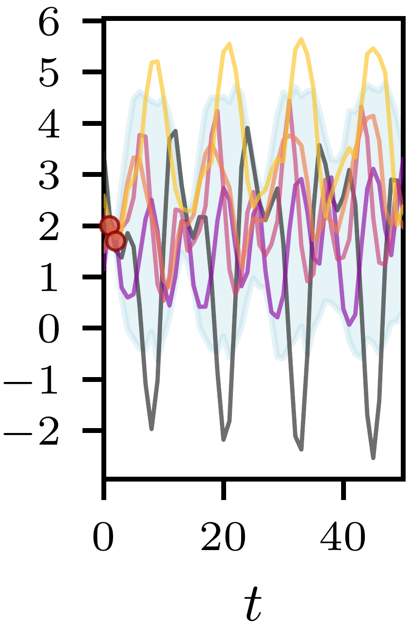
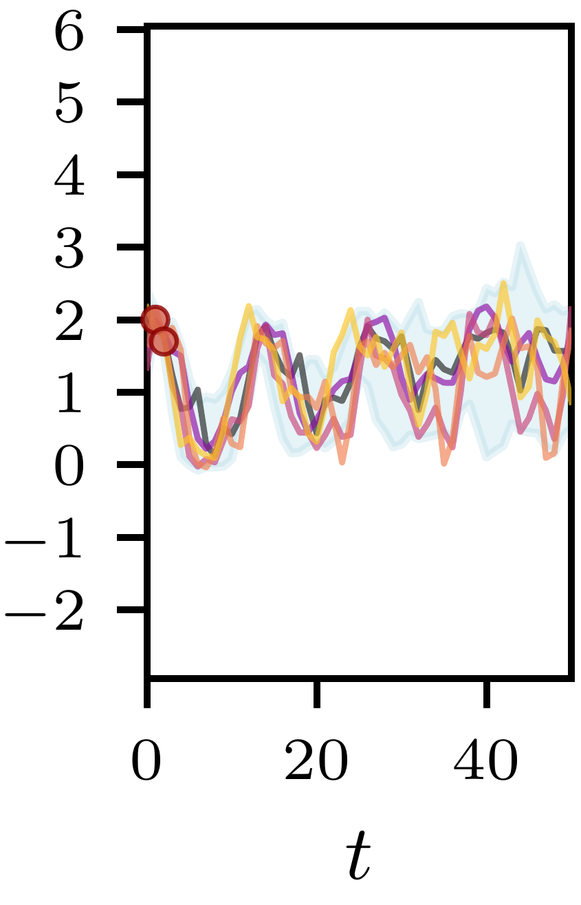
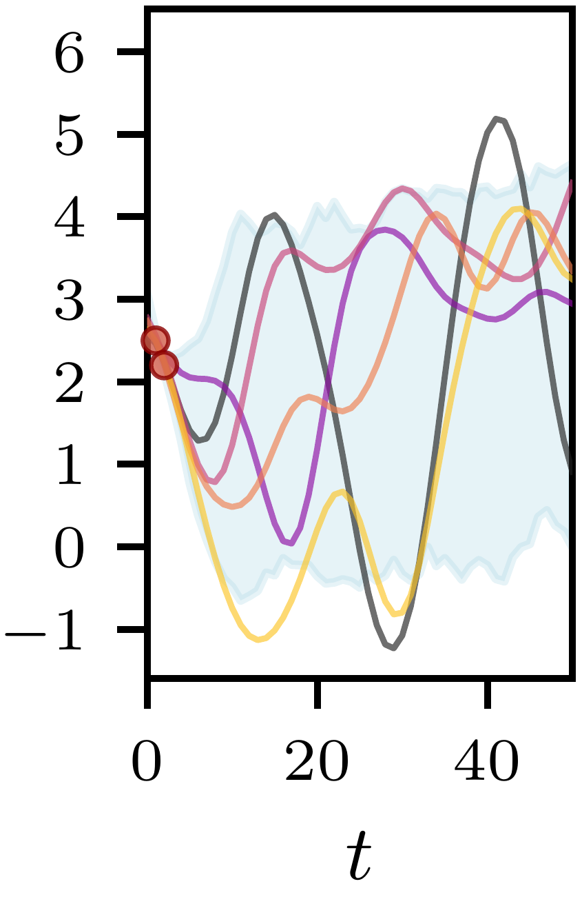
“Monthly average precipitation in San Diego in inches over 50 months, starting in January.”
What’s here and what’s next
We’ve done a lot of theory this year:
- Moss\(^*\), Astfalck\(^*\), …, Zammit-Mangion, Conditioning Gaussian Processes on Almost Anything, arXiv:2605.21041
- Sharrock, Astfalck, Moss, A General Framework for Conditioning Stochastic Processes, arXiv:2607.12922
- Zammit-Mangion, …, Astfalck, Spatial Prediction with Guided Diffusion, coming soon…
- Cowperthwaite, Astfalck, Sharrock, Moss, Scalable Gaussian Process Flows, coming soon…
- Riffel, Astfalck, Moss, Zammit-Mangion, Inference for Non-Ignorable Missingness with Diffusion Models, coming soon…
- Astfalck, …, Zammit-Mangion, Posterior Sampling by Likelihood-guided Diffusion of the Prior, coming soon…
Now, can we actually DO anything?!

Questions?
Slides and code: astfalckl.github.io/presentations
STREAM: unsw.edu.au/science/our-schools/maths/our-research/stream
l.astfalck@unsw.edu.au
Lachlan Astfalck | UNSW Spatio-Temporal Research for Environmental Analysis and Modelling