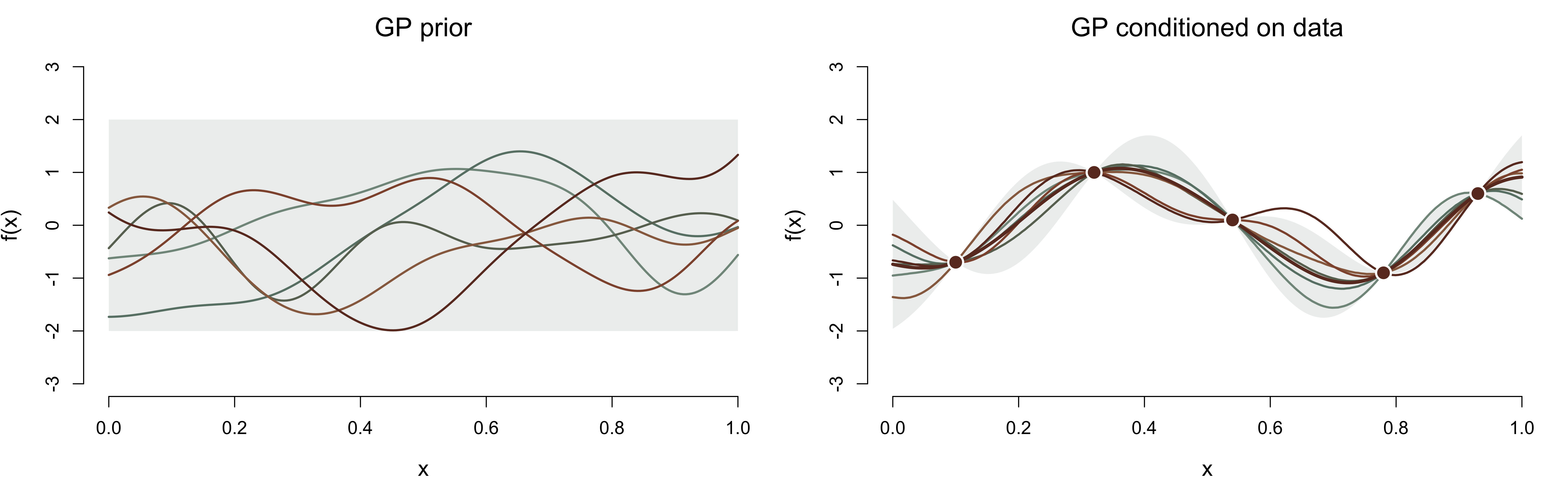
Conditioning Almost All Stochastic Processes
on Almost Anything

Lachlan Astfalck

UNSW Sydney | STREAM

2028-07-07

What problem are we solving?

• Assume a stochastic process prior \(f \sim \mathcal{SP}\) with \(f \in \mathcal{F}\) on domain \(x \in \mathcal{X}\)
• You want to update your prior on some information \(\mathcal{C}\)
  • maybe \(\mathcal{C}\) is observable data: \(y_i = g(f(x_i), \epsilon_i)\)
  • maybe \(\mathcal{C}\) asks for the stochastic process to be a solution to a PDE: \(\{f \in \mathcal{F} : \text{PDE is satisfied}\}\)
  • maybe \(\mathcal{C}\) asks for the stochastic process to be shape constrained, e.g. monotone: \(\{f \in \mathcal{F} : f(x_i) \leq f(x_j) \ \text{for all } x_i \leq x_j\}\)

How do we get \(p(f \mid \mathcal{C})\)?

Summary

Two papers:

• FlowGP — Conditioning Gaussian Processes on Almost Anything (Moss\(^*\), Astfalck\(^*\), …, Zammit-Mangion, arXiv:2605.21041)
• LatentFlow — A General Framework for Conditioning Stochastic Processes (Sharrock, Astfalck, Moss, arXiv:2607.12922)

Conditioning a stochastic process on non-linear, non-Gaussian, or weird information does not require MCMC, variational inference, or a trained neural network.

It requires a change of perspective borrowed from diffusion models.

A collection of caveats

• Here, we will assume finite dimensional \(\boldsymbol{f}_0 \in \mathbb{R}^d\).
• There are no neural networks (apart from in one funky application right at the end)
• I will not talk about hyperparameter inference
• Where the generator \(T_\vartheta\) isn’t differentiable, we can do some clever tricks
• There is an alternative ODE representation to everything in here, it’s bad for reasons I won’t discuss

All Cats Are Stochastic Processes

A cat is a random vector

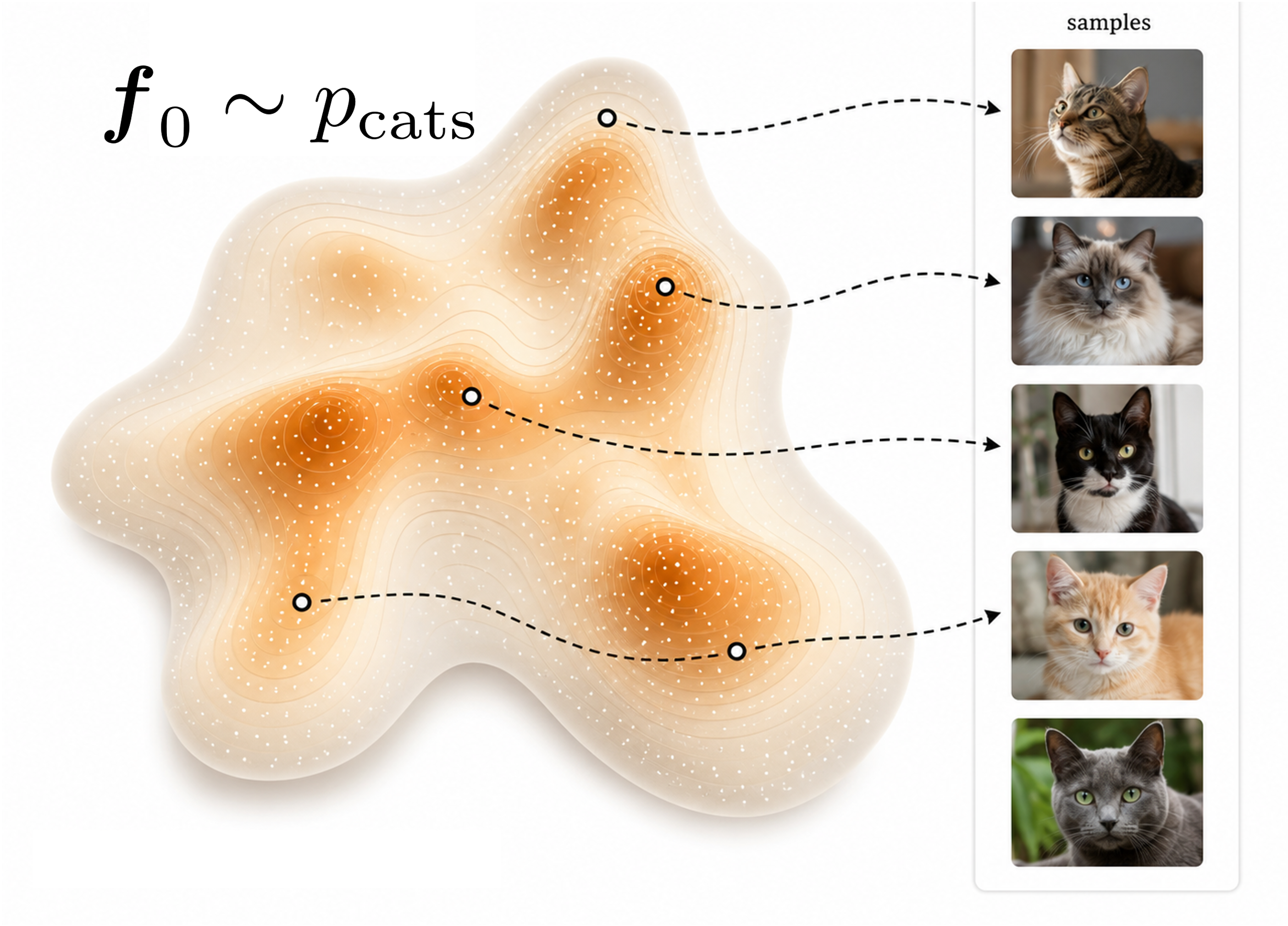
Diffusion modelling simply asks “how do I sample from an inconvenient distribution?”

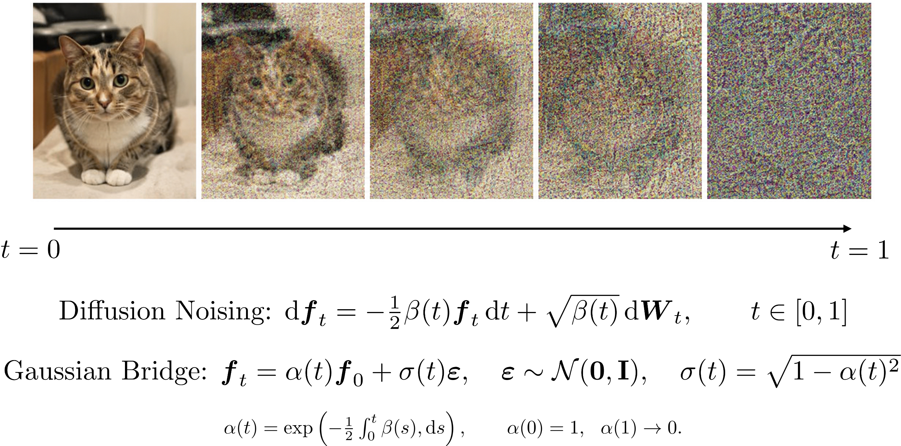
Noising a cat

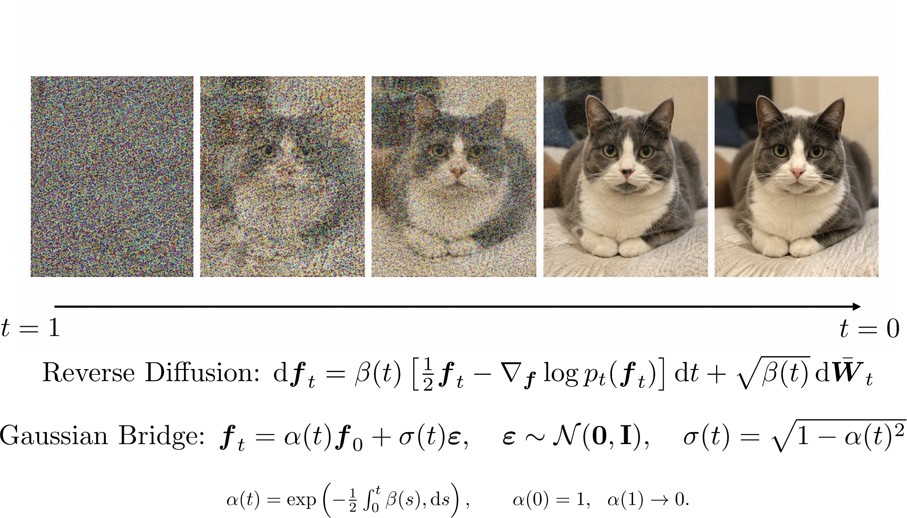
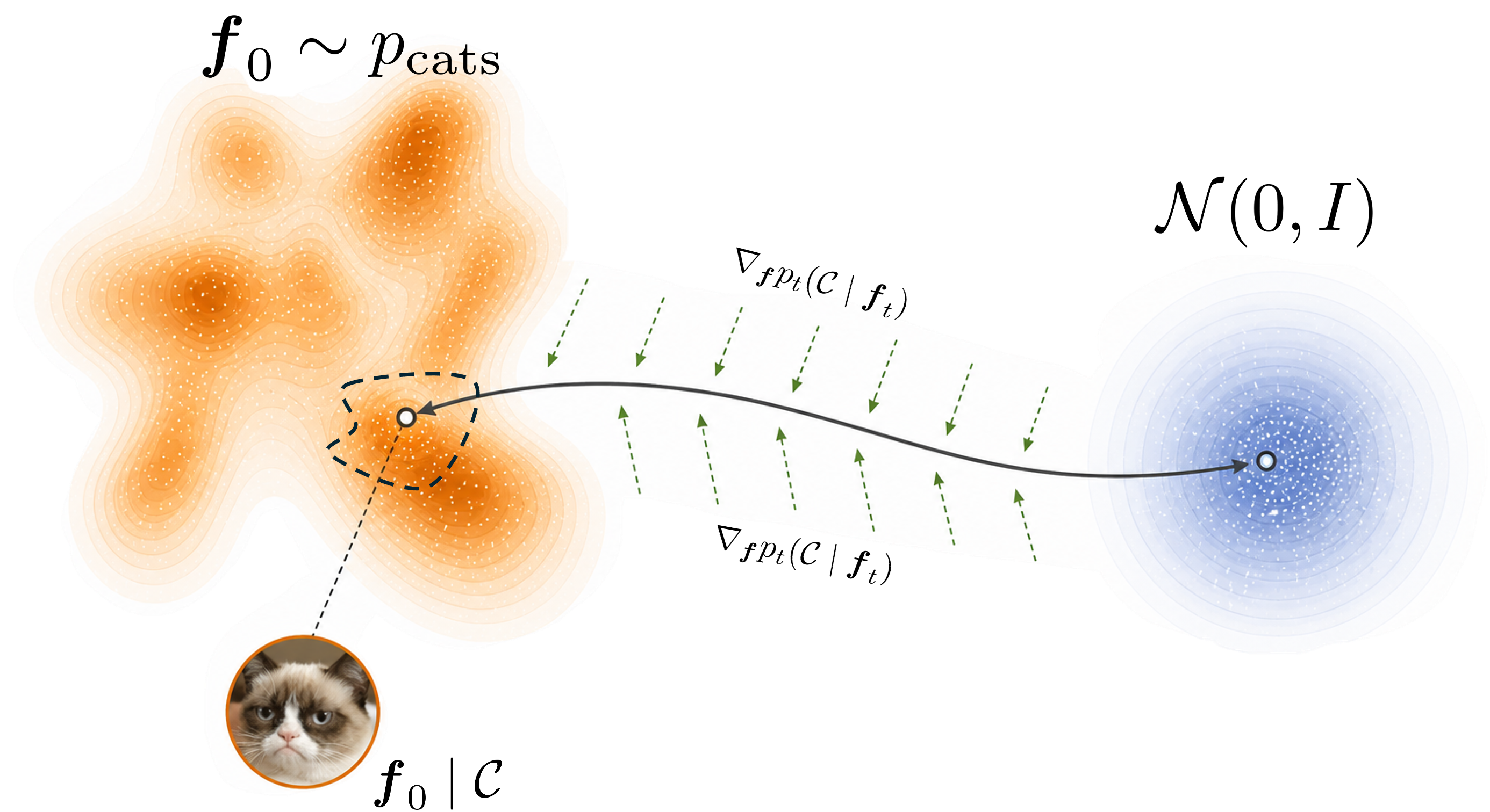
Reversing a cat

• The noising path is the marginal law of an SDE run forward.
• Write \(p_t\) for the marginal of \(\boldsymbol{f}_t\) — the law of the process after noising for time \(t\)
  • (so \(p_0 = p_\text{cat} = \mathcal{SP}\), \(p_1 \approx \mathcal{N}(\boldsymbol{0}, \mathbf{I})\))
• Anderson (1982) showed that the time reversal is also an SDE, \[\begin{aligned} \text{Forwards:}& \qquad \mathrm{d}\boldsymbol{f}_t = - \tfrac{1}{2}\beta(t) \boldsymbol{f}_t \mathrm{d}t + \sqrt{\beta(t)}\,\mathrm{d}\boldsymbol{W}_t. \\ \text{Backwards:}& \qquad \mathrm{d}\boldsymbol{f}_t = \beta(t)\left[\tfrac{1}{2}\boldsymbol{f}_t - \nabla_{\boldsymbol{f}}\log p_t(\boldsymbol{f}_t)\right]\mathrm{d}t + \sqrt{\beta(t)}\,\mathrm{d}\bar{\boldsymbol{W}}_t. \end{aligned}\]
• One unknown object: the time-dependent score \(\nabla_{\boldsymbol{f}} \log p_t\).
• If we know the score, noise flows backwards into cats.

Anderson (1982), Reverse-time diffusion equation models, Stochastic Processes and their Applications 12(3):313–326.

Reversing a cat

What does machine learning do?

• For cats, \(\nabla_\boldsymbol{f} \log p_t\) is unknown. Diffusion models learn it by fitting a network \(s_\theta(\boldsymbol{f}, t)\).
• That is the entire “ML” content of a diffusion model, everything else is stochastic calculus.
  • Find a few hundred million photos of cats
  • Noise them via the diffusion noising process
  • Train some \(s_\theta(\boldsymbol{f}, t) \approx \nabla_\boldsymbol{f} \log p_t\)
  • Sample from \(p_\text{cats}\) by pushing iid noise through the reverse diffusion

If we can obtain \(\nabla_\boldsymbol{f} \log p_t\), then we don’t need neural networks for the reverse diffusion

Conditional cats

• Want a grumpy cat? Bayes: \[ \nabla \log p_t(\boldsymbol{f}_0 \mid \mathcal{C} = \text{grumpy}) = \nabla \log p_t(\boldsymbol{f}_0) + \underbrace{\nabla \log p_t(\mathcal{C} = \text{grumpy} \mid \boldsymbol{f}_0)}_{\text{guidance}}. \]
• Add a likelihood term to the drift and the trajectory bends towards samples satisfying \(\mathcal{C}\). \[\mathrm{d}\boldsymbol{f}_t = \beta(t)\left[\tfrac{1}{2}\boldsymbol{f}_t - \nabla_{\boldsymbol{f}}\log p_t(\boldsymbol{f}_t \mid \mathcal{C})\right]\mathrm{d}t + \sqrt{\beta(t)}\,\mathrm{d}\bar{\boldsymbol{W}}_t\]
• In ML, this is called guidance. We will call it conditioning, because it is simply Bayes’ rule.
• Hold onto this for later.

Conditional cats

Stoch. Processes Are Boring Cats

A starting point, the Gaussian process

• A distribution over functions \(\boldsymbol{f}_0 : \mathcal{X} \to \mathbb{R}\), written \(\boldsymbol{f}_0 \sim \mathcal{GP}(m, k)\).
  • a mean function \(m(x) = \mathbb{E}[\boldsymbol{f}_0(x)]\) — usually taken \(\equiv 0\);
  • a covariance kernel \(k(x, x') = \mathrm{Cov}\big(\boldsymbol{f}_0(x), \boldsymbol{f}_0(x')\big)\) — how much the values at \(x\) and \(x'\) move together.
• Defining property: at any finite set of inputs \(x_1, \dots, x_n\), the function values are jointly Gaussian, \[ \big(\boldsymbol{f}_0(x_1), \dots, \boldsymbol{f}_0(x_n)\big) \sim \mathcal{N}(\boldsymbol{m}, \mathbf{K}), \qquad \mathbf{K}_{ij} = k(x_i, x_j). \]

A GP is just a multivariate normal over infinitely many index points.

Conditioning a Gaussian process

• Put a GP prior on \(f\), observe data, get a GP posterior — this is Gaussian process regression.
• With linear-Gaussian observations \(\boldsymbol{y} = \mathbf{L}\boldsymbol{f}_0 + \boldsymbol{\varepsilon}\), the posterior is closed form: \[ \begin{aligned} \mathbf{m}_{*|\boldsymbol{y}} &= \mathbf{m}_* + \mathbf{K}_{**}\mathbf{L}^{\mathsf{T}}\!\left(\mathbf{L}\mathbf{K}_{**}\mathbf{L}^{\mathsf{T}} + \boldsymbol{\Gamma}\right)^{-1}\!(\boldsymbol{y} - \mathbf{L}\mathbf{m}_*),\\ \mathbf{K}_{**|\boldsymbol{y}} &= \mathbf{K}_{**} - \mathbf{K}_{**}\mathbf{L}^{\mathsf{T}}\!\left(\mathbf{L}\mathbf{K}_{**}\mathbf{L}^{\mathsf{T}} + \boldsymbol{\Gamma}\right)^{-1}\!\mathbf{L}\mathbf{K}_{**}. \end{aligned} \]

Prior samples → posterior samples through the dots is the mental picture; the formulas are the “comfort object”. Then name the wall everyone has hit: conjugacy is the boundary of exactness.

A GP is a diffusion where everything is analytic

Take the diffusion machinery from Section 1 and set the target to a GP. The marginal \(p_t\) stays Gaussian, and every piece is known in closed form: \[ p_t = \mathcal{N}\big(\boldsymbol{b}(t),\, \mathbf{A}(t)\big), \qquad \boldsymbol{b}(t) = \alpha(t)\,\mathbf{m}_*, \qquad \mathbf{A}(t) = \alpha^2(t)\mathbf{K}_{**} + (1-\alpha^2(t))\mathbf{I}. \] The score is closed form, no neural networks: \[ \nabla_{\boldsymbol{f}}\log p_t(\boldsymbol{f}_t) = -\mathbf{A}(t)^{-1}\big(\boldsymbol{f}_t - \boldsymbol{b}(t)\big). \] Drop it straight into the reverse-time SDE and integrate from \(t=1\) to \(t=0\): \[ \mathrm{d}\boldsymbol{f}_t = \beta(t)\left[\tfrac{1}{2}\boldsymbol{f}_t - \nabla_{\boldsymbol{f}}\log p_t(\boldsymbol{f}_t)\right]\mathrm{d}t + \sqrt{\beta(t)}\,\mathrm{d}\bar{\boldsymbol{W}}_t. \]

A GP is a very boring cat. It’s just a diffusion model whose score you can write down.

Watch it happen

Whitening into better coordinates

“The most efficient thing for a computer to do is nothing” - Prof. Philipp Hennig

Whiten: \(\hat{\boldsymbol{f}}_0 = \mathbf{K}_{**}^{-1/2}(\boldsymbol{f}_0 - \mathbf{m}_*)\), the dynamics vanish entirely … the linear drift term is zero.

Gaussianity was never the point

• What did we actually do? We rotated the space by some deterministic \(T_\vartheta^{-1} = \mathbf{K}_{**}^{-1/2}\).
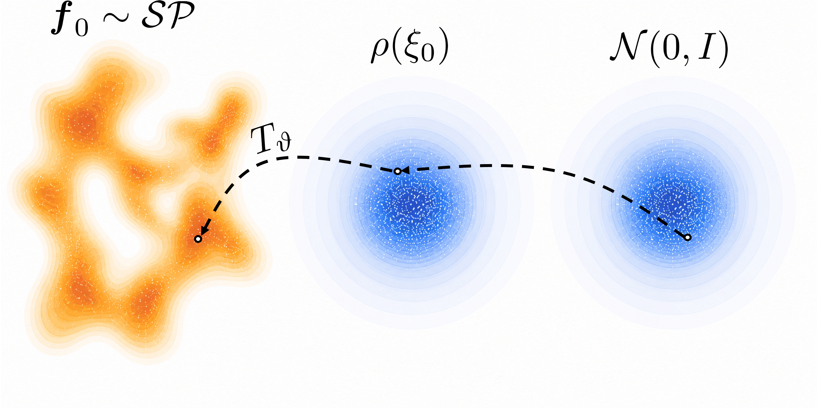
• The only property we require to do this trick is a deterministic map of simple noise, \[ \boldsymbol{f}_0 = T_\vartheta(\boldsymbol{\xi}_0), \qquad T_\vartheta : \mathbb{R}^{m} \to \mathbb{R}^{d}, \qquad \boldsymbol{\xi}_0 \sim \mathcal{N}(\boldsymbol{0}, \mathbf{I}_m). \]
  • the latent \(\boldsymbol{\xi}_0\) need not match \(\boldsymbol{f}_0\) in size (\(m \neq d\) in general)
• Rosenblatt (1952): after discretisation, essentially every process admits such a representation.
• For a GP, \(T_\vartheta = \mathbf{K}_{**}^{1/2}\) is the affine whitening map (here \(m = d\)).
• For everything else, \(T_\vartheta\) is … whatever your simulator already does.

Rosenblatt (1952), Remarks on a multivariate transformation, The Annals of Mathematical Statistics 23(3):470–472.

The hinge of the talk. The latent innovation representation, not Gaussianity, is the real requirement — this is LatentFlow’s key observation.

A gallery of boring cats

Every one is \(\boldsymbol{f}_0 = T_\vartheta(\boldsymbol{\xi}_0)\) for a tractable generator \(T_\vartheta\) and iid-normal latent \(\boldsymbol{\xi}_0\):

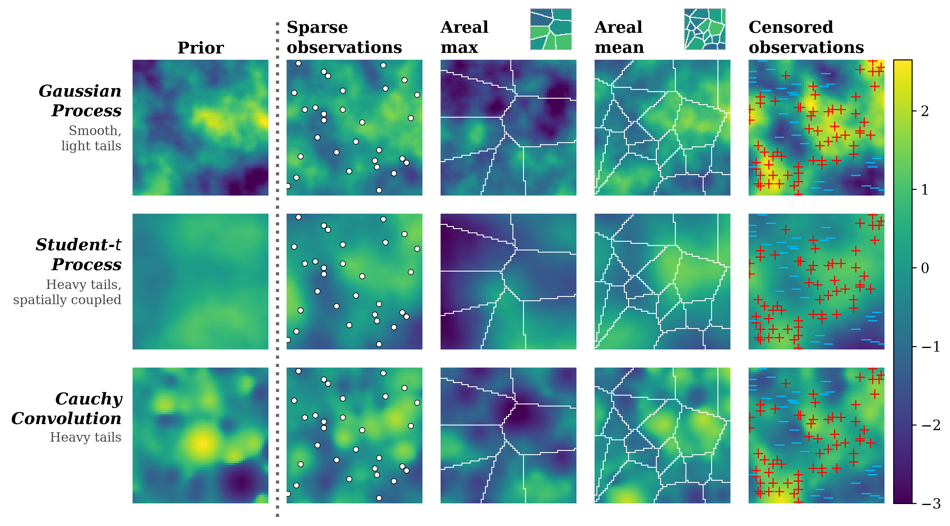
• Gaussian & heavy-tailed fields — GP, Student-\(t\), Cauchy convolution, max-stable: Gaussian innovations \(\times\) a scale / mixing variable.
• Discrete fields — Potts (\(q\) states): ordered-domain labels from latent noise.
• SDEs — life & physical sciences — Ornstein–Uhlenbeck, Heston (stochastic volatility), SIR (epidemics), Lotka–Volterra (predator–prey), FitzHugh–Nagumo (neurons): \(T_\vartheta\) is the Euler–Maruyama solver, \(\boldsymbol{\xi}_0\) its driving increments.
• SPDEs — spatio-temporal — Allen–Cahn phase fields (122K dims), advection–diffusion plumes (160 dims), FitzHugh–Nagumo media (40K dims).

If you can simulate it from noise, it qualifies. Your existing simulator is already \(T_\vartheta\).

Breadth slide — really flex the menagerie. Punchline: nothing needs rebuilding; the generator you already have IS the map. Land it fast, one beat per line.

For example: the Student-\(t\) process

• A Student-\(t\) process \(f \sim \mathcal{TP}_\nu(m_\vartheta, k_\vartheta)\) is a GP with one random global scale — heavy tails, spatially coupled.
• Draw it as a scale mixture of Gaussians, with \(\mathbf{L}_\vartheta\mathbf{L}_\vartheta^{\mathsf T} = \mathbf{K}_\vartheta\): \[ \boldsymbol{f}_0 = m_\vartheta + \omega^{-1/2}\,\mathbf{L}_\vartheta\,\boldsymbol{v}, \qquad \boldsymbol{v} \sim \mathcal{N}(\boldsymbol{0}, \mathbf{I}_m), \quad \omega \sim \mathrm{Gamma}\!\big(\tfrac{\nu}{2}, \tfrac{\nu}{2}\big). \]
• Push the scale onto a standard normal too — with \(a \sim \mathcal{N}(0,1)\) and \(G_\nu(a) = F_{\Gamma,\nu}^{-1}\!\big(\Phi(a)\big)\): \[ \boldsymbol{f}_0 = T_\vartheta(\boldsymbol{\xi}_0) = m_\vartheta + G_\nu(a)^{-1/2}\,\mathbf{L}_\vartheta\,\boldsymbol{v}, \qquad \boldsymbol{\xi}_0 = (\boldsymbol{v}, a) \sim \mathcal{N}(\boldsymbol{0}, \mathbf{I}_{m+1}). \]

\(m\) Gaussian innovations make the field; one more makes the heavy tail. The whole process is a deterministic map of \(m{+}1\) iid normals.

Concrete instance of the general framework. \(\Phi\) is the standard-normal CDF, \(F_{\Gamma,\nu}\) the Gamma\((\nu/2,\nu/2)\) CDF, so \(G_\nu(a)\) is a Gamma draw pushed through a normal — the scale variable rewritten as a function of one more iid normal. Everything is now \(T_\vartheta\) of standard noise, exactly as the gallery promised.

Where we stand

• Push \(\boldsymbol{\xi}_0 \sim \mathcal{N}(\boldsymbol{0},\mathbf{I})\) through \(T_\vartheta\)
• This gives marginal samples of nearly any stochastic process. (We could already do this, it’s just simulation.)
• The score of the latent noising process with respect to \(\boldsymbol{\xi}_t\) is closed form.
• Thus the boring-cat property survives in latent space for every process in the gallery.

• Now we need a framework for conditioning…

Grumpy Stochastic Processes

Guidance is just Bayes

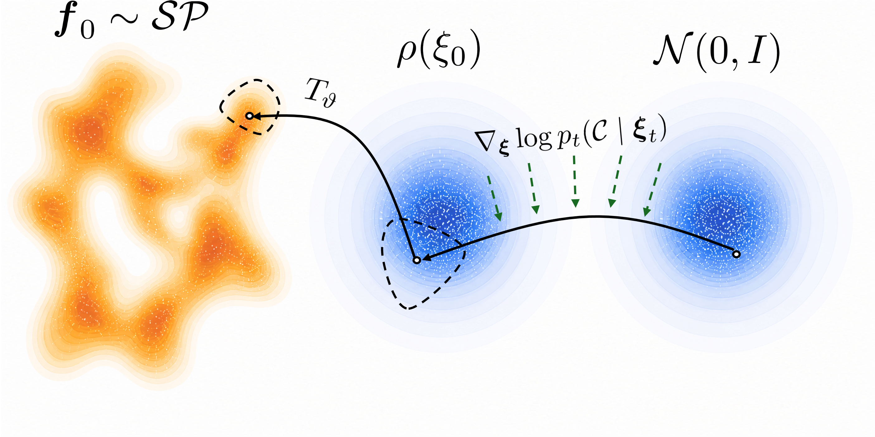
We work in latent space. Target the pulled-back posterior: \[ \pi(\boldsymbol{\xi}_0 \mid \mathcal{C}) \propto p\big(\mathcal{C} \mid T_\vartheta(\boldsymbol{\xi}_0)\big) \rho(\boldsymbol{\xi}_0). \]

Along the latent flow, the score decomposes: \[ \nabla_{\boldsymbol{\xi}} \log p_t(\boldsymbol{\xi}_t \mid \mathcal{C}) = \underbrace{\nabla_{\boldsymbol{\xi}} \log p_t(\boldsymbol{\xi}_t)}_{=\,-\boldsymbol{\xi}_t\ \text{(exact)}} + \underbrace{\nabla_{\boldsymbol{\xi}} \log p_t(\mathcal{C} \mid \boldsymbol{\xi}_t)}_{\text{guidance}}. \]

Run the same SDE in \(\boldsymbol{\xi}\)-space, add the guidance term, then push through \(T_\vartheta\).

The latent prior is exact at every \(t\). Guidance is the only thing to approximate.

And for us, guidance is somewhat tractable

We need \(\nabla_{\boldsymbol{\xi}} \log p_t(\mathcal{C}\mid\boldsymbol{\xi}_t) = \nabla_{\boldsymbol{\xi}} \log \int p\big(\mathcal{C} \mid T_\vartheta(\boldsymbol{\xi}_0)\big) \, p(\boldsymbol{\xi}_0 \mid \boldsymbol{\xi}_t)\,\mathrm{d}\boldsymbol{\xi}_0.\)

As \(p(\boldsymbol{\xi}_0 \mid \boldsymbol{\xi}_t)\) is tractable and we can importance-sample: \[ \nabla_{\boldsymbol{\xi}}\log p_t(\mathcal{C}\mid \boldsymbol{\xi}_t) \approx \alpha(t) \sum_{i=1}^{S} \bar{w}^{(i)}\, \nabla_{\boldsymbol{\xi}}\log p\big(\mathcal{C}\mid T_\vartheta(\boldsymbol{\xi}_0^{(i)})\big), \qquad \bar w^{(i)} \propto p\big(\mathcal{C}\mid T_\vartheta(\boldsymbol{\xi}_0^{(i)})\big). \] The last gradient is just the chain rule through the generator: \[ \nabla_{\boldsymbol{\xi}}\log p\big(\mathcal{C}\mid T_\vartheta(\boldsymbol{\xi}_0)\big) = \underbrace{\big[\partial_{\boldsymbol{\xi}} T_\vartheta(\boldsymbol{\xi}_0)\big]^{\!\mathsf T}}_{\text{Jacobian of the generator}}\, \nabla_{\boldsymbol{f}_0}\log p(\mathcal{C}\mid\boldsymbol{f}_0). \]

(There are some issues with weight-degeneracy in importance sampling that don’t seem to matter to us for a handful of esoteric reasons.)

Marginal Sampling

Conditional Sampling

Error, approximations & computation

	Error source	For cats	For us
1	Marginal score \(\nabla\log p_t\)	uncontrolled	exact
2	Guidance approximation	uncontrolled	explicit; \(\mathcal{O}(S^{-1})\) bias
3	Discretisation	controllable	solver order \(h^q\), same bound

• Per sample: one reverse-SDE solve (no mixing time or training)
• Parallelises trivially (all shown examples are milliseconds to a few seconds each, on a CPU)

We are not cheapening a hard computation. This will not somehow make computationally prohibitive processes (with respect to marginal sampling) easier.

Silly Benchmarking Problems

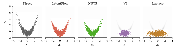
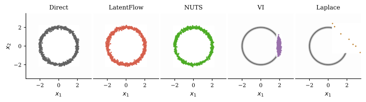
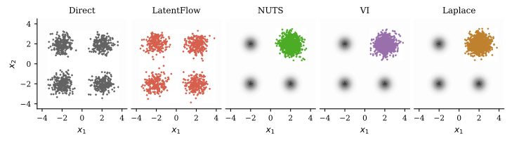
Shape & physics constrained GPs

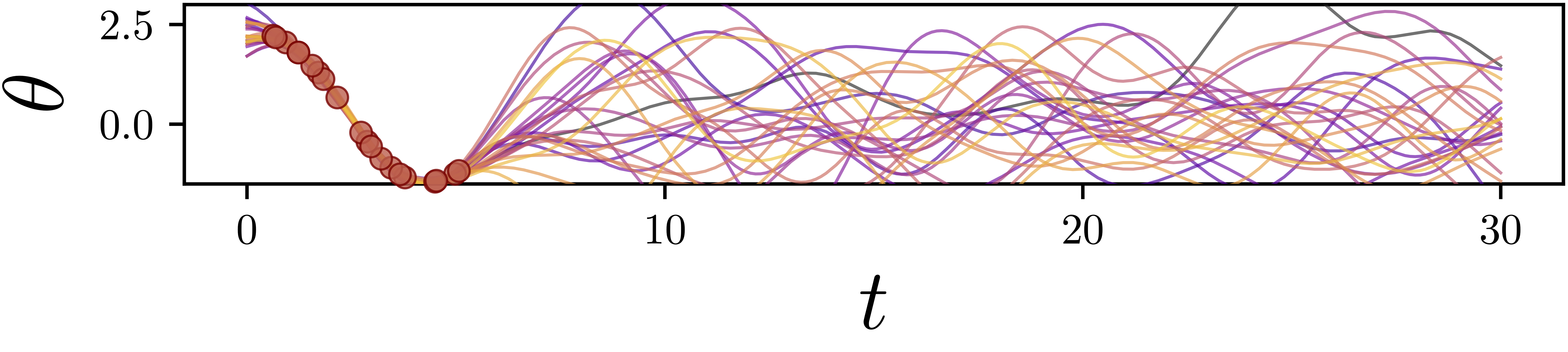
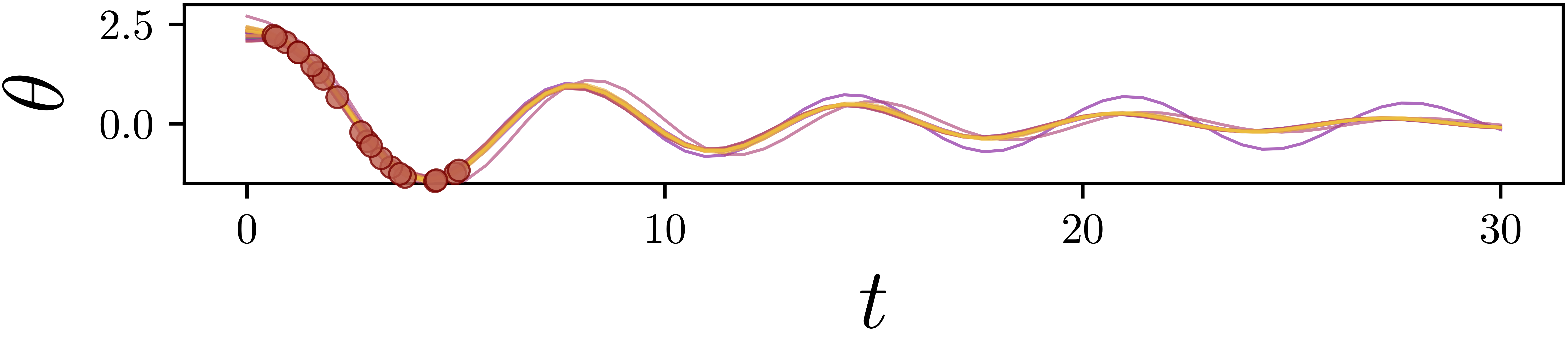
Temporal processes

Spatial processes

Spatio-temporal SPDEs

Conditioning on Natural Language

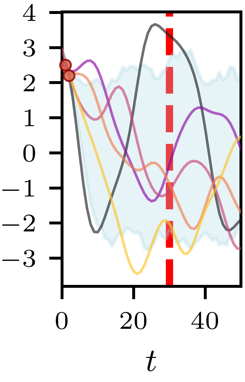
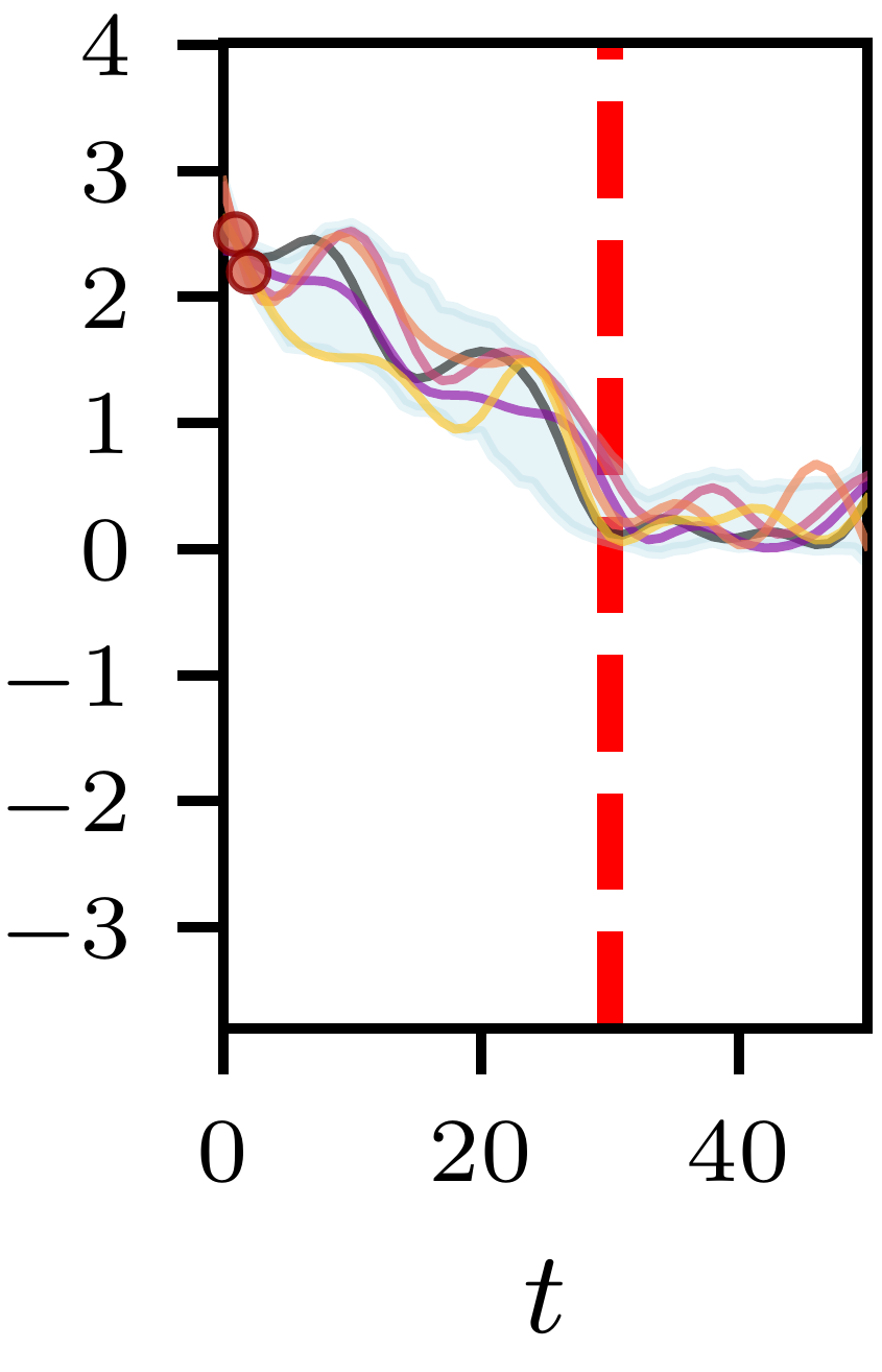
“A small UK company’s daily stock price in GBP over 50 trading days. On day 30 the company enters compulsory liquidation and is permanently delisted from the London Stock Exchange.”

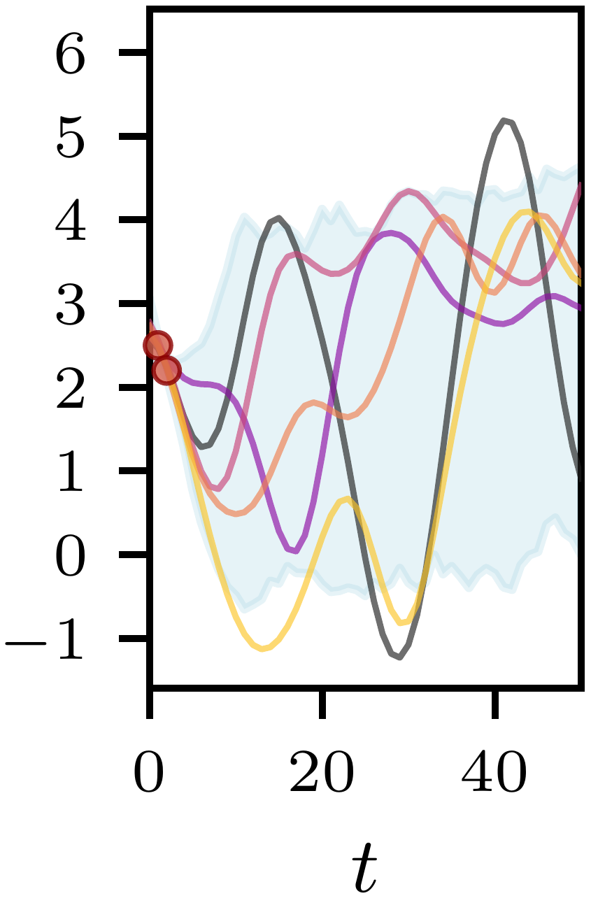
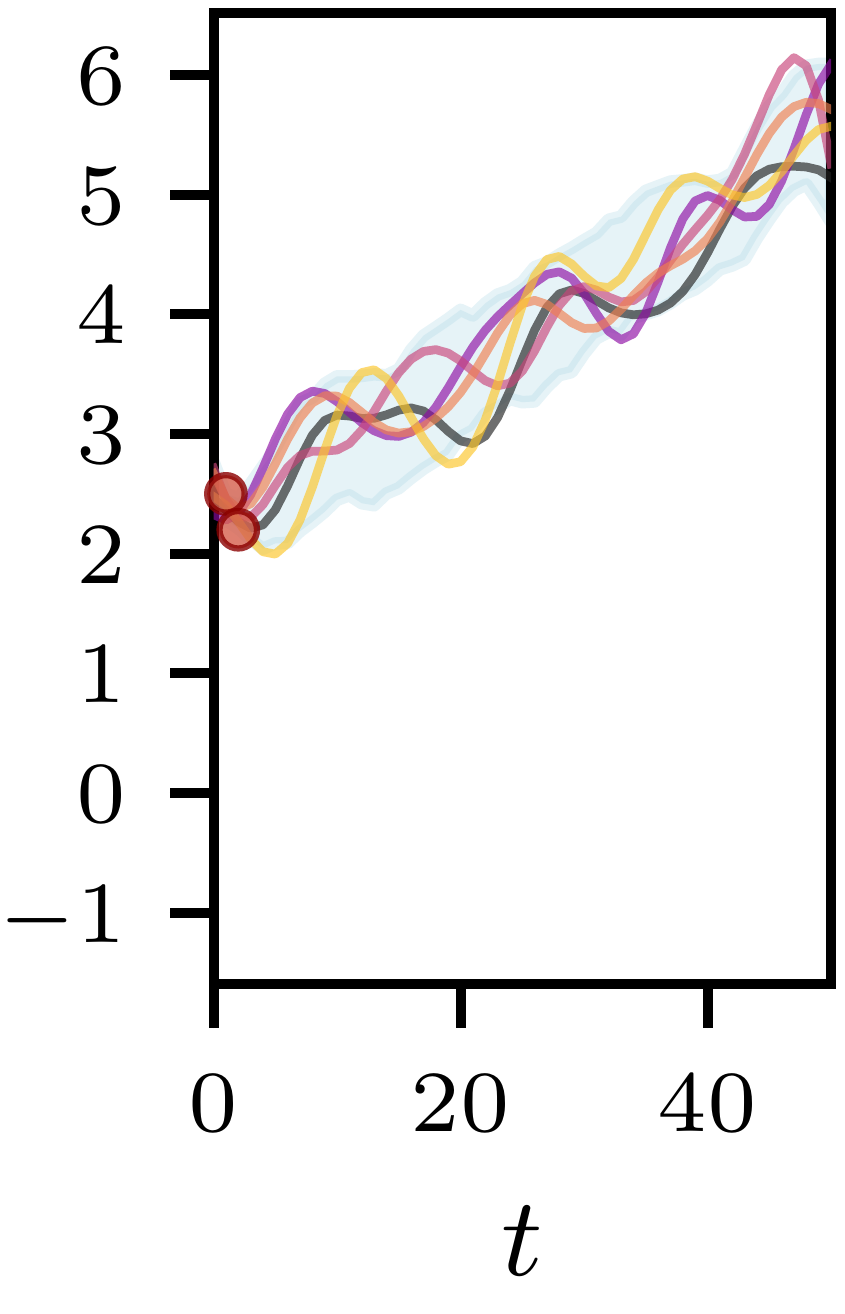
“A small UK company’s daily stock price in GBP over 50 trading days. The company has no notable news during the period, but performs well. Ending with a value over 5 GBP per share.”

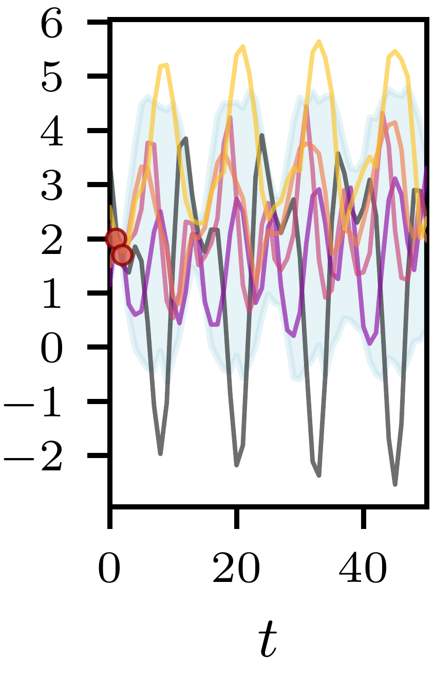
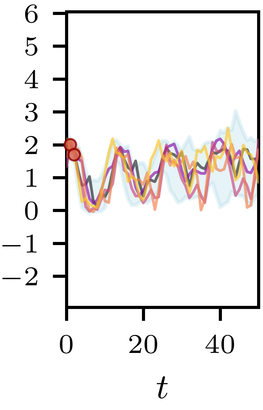
“Monthly average precipitation in San Diego in inches over 50 months, starting in January.”

Questions?

Slides and code: astfalckl.github.io/presentations

STREAM: unsw.edu.au/science/our-schools/maths/our-research/stream

l.astfalck@unsw.edu.au