ML with Gaussian Likelihood • bskernel

We begin by illustrating a simple example of fitting an ACF to simulated time-series data using maximum likelihood. We simulate a stationary Gaussian process with a known Matérn-3/2 auto-covariance structure. Then, we fit an auto-covariance model using the bskernel package, assuming linear ( $k=1$ ) B-spline spectral basis. The resulting estimated ACF is compared to the true model.

In what follows, as we sample our data regularly, we use Toeplitz tricks to speed matters up. Generalising to non-regular data is trivial, it will just take longer for the optimiser to compute.

Simulate a Gaussian process with known autocovariance

Most of this is standard; we lean on the package SuperGauss to efficiently sample the GP and set fft = FALSE so that this sample is an exact draw.

library(bskernel)
library(dplyr)
library(SuperGauss)

matern32_cov <- function(d, range, sigma2) {
  sqrt3_d <- sqrt(3) * d / range
  sigma2 * (1 + sqrt3_d) * exp(-sqrt3_d)
}

n <- 2000
n_knots <- 4
range <- 2
k <- 1
b <- 0.1

tau <- 0:(n - 1)
mat32_acf <- matern32_cov(tau, range, sigma2 = 1)

y <- SuperGauss::rnormtz(n = 1, mat32_acf, fft = FALSE)

Estimate the ACF using spline kernels

There are a couple of things to note here. First, the data are sampled regularly with spacing 1, so the Nyquist frequency is 0.5. We extend the knot spacing past this as we are using linear basis. Same with the first knot, we are creating a symmetry about 0. Next, optim_toeplitz_mle is optimising over the log space of the parameters, hence why we must exponentiate the optimiser output. Constraining the parameters to be positive like this is a sufficient but not necessary condition to yield a positive semi-definite estimate. Finally, the easiest way to symmetrise the bases defined by the knots is to just take the real values.

The plot of the estimated vs true ACF is given below.

knots <- c(-0.05, 0, 0.05, 0.1, 0.2, 0.3, 0.5, 0.7)
c_init <- c(0.3, 0.2, 0.15, 0.15, 0.1, 0.1)

log_c_mle <- optim_toeplitz_mle(c_init, knots, k, y)$par
c_mle <- exp(log_c_mle)
acf_est <- reconstruct_acf(c_mle, knots, k, tau) %>% Re()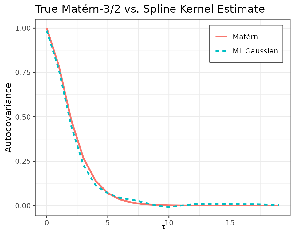

Gradient of the Toeplitz Representation

Warning: mathematical details not required to run the code.

This optimisation runs efficiently in part as we have baked in the gradient using the Toeplitz representation of the likelihood. See compute_toeplitz_loglik_grad if you want to unpack this.

Let $\mathbf{y} \in \mathbb{R}^n$ be a zero-mean stationary Gaussian process with Toeplitz covariance matrix $\Sigma = T(\boldsymbol{\rho})$ where $T(\boldsymbol{\rho})$ is a symmetric Toeplitz matrix defined by the autocovariance vector $\boldsymbol{\rho} = (\rho_0, \rho_1, \dots, \rho_{n-1})$ . We model each autocovariance entry as $\rho_\tau = \sum_{i=0}^{m-1} c_i \, \phi_i(\tau)$ where

$c_i$ are coefficients,
$\phi_i(\tau)$ is the inverse Fourier transform of the $i$ -th B-spline spectral basis function (eqn 5 of the paper).

The log-likelihood is $\ell(\mathbf{c}) = -\frac{1}{2} \left[ n \log(2\pi) + \log |\Sigma(\mathbf{c})| + \mathbf{y}^\top \Sigma(\mathbf{c})^{-1} \mathbf{y} \right].$

Apply the chain rule, $\frac{\partial \ell}{\partial c_i} = \sum_{\tau=0}^{n-1} \frac{\partial \ell}{\partial \rho_\tau} \cdot \frac{\partial \rho_\tau}{\partial c_i}.$ From standard matrix calculus, $\frac{\partial \ell}{\partial \rho_\tau} = \frac{1}{2} \left[ \mathbf{y}^\top \Sigma^{-1} J^\tau \Sigma^{-1} \mathbf{y} - \operatorname{tr}(\Sigma^{-1} J^\tau) \right]$ where $J^\tau$ is the Toeplitz matrix with 1s on the $\tau$ -th (symmetric) off-diagonal, and 0 elsewhere. In practice, this is efficiently handled by the SuperGauss::NormalToeplitz class. Since, $\rho_\tau = \sum_i c_i \, \phi_i(\tau) \quad \Rightarrow \quad \frac{\partial \rho_\tau}{\partial c_i} = \phi_i(\tau),$ the Jacobian $\partial \boldsymbol{\rho} / \partial \mathbf{c} \in \mathbb{R}^{n \times K}$ has entries $\left[ \frac{\partial \boldsymbol{\rho}}{\partial \mathbf{c}} \right]_{\tau,i} = \phi_i(\tau).$

Putting it together, $\nabla_{\mathbf{c}} \ell(\mathbf{c}) = \left( \frac{\partial \ell}{\partial \boldsymbol{\rho}} \right)^\top \cdot \left( \frac{\partial \boldsymbol{\rho}}{\partial \mathbf{c}} \right).$ In code, SuperGauss handles this all beautifully with

grad <- nt$grad(z = y, dz = matrix(0, n, n_basis), acf = rho, dacf = dacf)

Lastly, if we optimise over the log-parameters $\theta_i = \log c_i$ , the chain rule gives $\frac{\partial \ell}{\partial \theta_i} = \frac{\partial \ell}{\partial c_i} \cdot \frac{\partial c_i}{\partial \theta_i} = \frac{\partial \ell}{\partial c_i} \cdot c_i$ and so in code,

grad_theta <- grad * c