ML with Whittle Likelihood

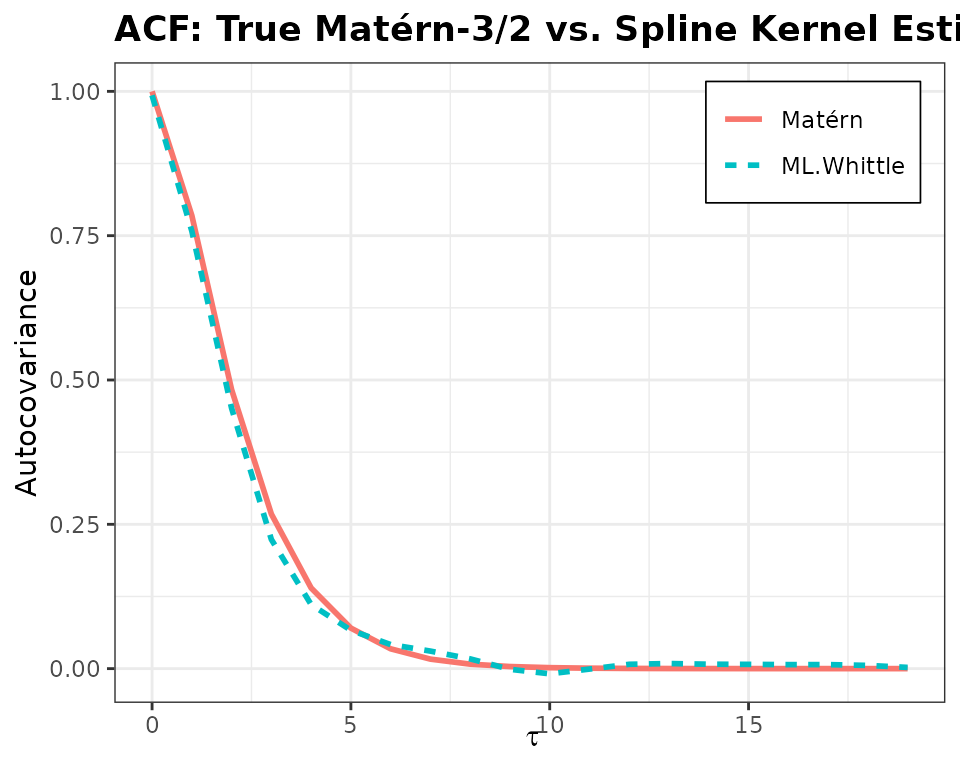
We now provide a simple example of fitting an ACF to simulated time-series data by maximising Whittle’s likelihood, a pseudo-likelihood that approximates the Gaussian likelihood in the Fourier domain. As discussed in the paper, this is particularly natural in fitting the spline kernels.

As before, we simulate a stationary Gaussian process with a known Matérn-3/2 auto-covariance structure, and as again, we fit an auto-covariance model using the bskernel package, assuming linear ($k=1$) B-spline spectral basis.

To use Whittle’s likelihood, we require regularly sampled data, and so it is natural to use Toeplitz methods to speed up simulation. In what follows, I call the occasional function from speccy, this is some of my other software designed to handle a bunch of spectral/Fourier methods.

---

Simulate a Gaussian process with known autocovariance

Most of this is standard; we lean on the package SuperGauss to efficiently sample the GP and set fft = FALSE so that this sample is an exact draw. We then calculate the periodogram, note it’s values are double here as we are only going to consider the folded periodogram in the positive frequencies, and we drop the 0th frequency element as it does behave well with Whittle’s likelihood.

library(bskernel)
library(dplyr)
library(SuperGauss)
library(speccy)

matern32_cov <- function(d, range, sigma2) {
  sqrt3_d <- sqrt(3) * d / range
  sigma2 * (1 + sqrt3_d) * exp(-sqrt3_d)
}

n <- 2000
n_knots <- 4
range <- 2
k <- 1
b <- 0.1

tau <- 0:(n - 1)
mat32_acf <- matern32_cov(tau, range, sigma2 = 1)

y <- SuperGauss::rnormtz(n = 1, mat32_acf, fft = FALSE)

I <- 2 * speccy::periodogram(y)$estimate[-1]
omegas <- speccy::periodogram(y)$ff[-1]

---

Estimate the ACF using Whittle’s likelihood

This runs similar as the Gaussian likelihood case, except, now, we are optimising the bases in the Fourier domain directly. The only potentially odd thing to note about this is how the basis matrix is formed, effectively, I’m folding the negative frequencies into the positive, and then we are going to fit to the positive frequencies.

knots <- c(-0.05, 0, 0.05, 0.1, 0.2, 0.3, 0.5, 0.7)
c_init <- c(0.3, 0.2, 0.15, 0.15, 0.1, 0.1)

B_pos <- build_bspline_design_matrix(omegas, knots = knots, k = k)
B_neg <- build_bspline_design_matrix(-omegas, knots = knots, k = k)
B <- B_pos + B_neg

c_whittle <- optim_whittle(omegas, I, B, c0 = c_init)$c
acf_est <- Re(reconstruct_acf(c_whittle, knots, k, tau))